Detection of Crop Seeding and Harvest through Analysis of Time-Series Sentinel-1 Interferometric SAR Data

Abstract

Synthetic aperture radar (SAR) is more sensitive to the dielectric properties and structure of the targets and less affected by weather conditions than optical sensors, making it more capable of detecting changes induced by management practices in agricultural fields. In this study, the capability of C-band SAR data for detecting crop seeding and harvest events was explored. The study was conducted for the 2019 growing season in Temiskaming Shores, an agricultural area in Northern Ontario, Canada. Time-series SAR data acquired by Sentinel-1 constellation with the interferometric wide (IW) mode with dual polarizations in VV (vertical transmit and vertical receive) and VH (vertical transmit and horizontal receive) were obtained. interferometric SAR (InSAR) processing was conducted to derive coherence between each pair of SAR images acquired consecutively in time throughout the year. Crop seeding and harvest dates were determined by analyzing the time-series InSAR coherence and SAR backscattering. Variation of SAR backscattering coefficients, particularly the VH polarization, revealed seasonal crop growth patterns. The change in InSAR coherence can be linked to change of surface structure induced by seeding or harvest operations. Using a set of physically based rules, a simple algorithm was developed to determine crop seeding and harvest dates, with an accuracy of 85% (n = 67) for seeding-date identification and 56% (n = 77) for harvest-date identification. The extra challenge in harvest detection could be attributed to the impacts of weather conditions, such as rain and its effects on soil moisture and crop dielectric properties during the harvest season. Other factors such as post-harvest residue removal and field ploughing could also complicate the identification of harvest event. Overall, given its mechanism to acquire images with InSAR capability at 12-day revisiting cycle with a single satellite for most part of the Earth, the Sentinel-1 constellation provides a great data source for detecting crop field management activities through coherent or incoherent change detection techniques. It is anticipated that this method could perform even better at a shorter six-day revisiting cycle with both satellites for Sentinel-1. With the successful launch (2019) of the Canadian RADARSAT Constellation Mission (RCM) with its tri-satellite system and four polarizations, we are likely to see improved system reliability and monitoring efficiency.

1. Introduction

There is an increasing need for continuous monitoring of crop growth conditions and its response to environment and management activities for the development and assessment of best management practices (BMP). The Food and Agriculture Organization (FAO) of the United Nations has set out the 2030 Agenda of transforming the world through food and agriculture [1]. With an increasing emphasis on sustainable agriculture, the metrics of land management activities throughout the life cycle of crop production become even more important, especially in the context of climate change. In-season information on the onset of key stages of crop production, from soil preparation, seeding to harvest, as well as crop residue management, is of great value to a wide range of user communities, including producers, agri-food, and renewable energy industry, commodity trade board, and crop modelers. Information on land management activities is also key to evaluating environmental footprint resulted from crop production [2,3,4].

Earth observation (EO) data have long been used for land cover and land use mapping. In particular, free-access optical satellite data, such as Moderate Resolution Imaging Spectroradiometer (MODIS) and Landsat data, have been extensively used for agricultural applications at local, regional and global scales. The most frequent applications are using EO data for crop type mapping using various image classification methods. Because crops are affected by seasonal growth patterns, continuous observation is needed to track the growing conditions, particularly during critical phenological stages. The short revisit time of the MODIS sensor allows for crop emergence detection and seeding date estimation [5,6,7], however the spatial resolution of the data is relatively coarse for field-level applications. Given the many benefits of the optical sensors, there are still three inherent shortcomings, e.g., data acquisition is susceptible to interference by weather conditions (e.g., cloud cover), data is insensitive to crop structure and soil disturbances, and signal saturates when vegetation biomass is high. These shortcomings limit the operational applications of optical EO in agriculture, because fields are frequently managed and crops vary continuously throughout the growing season [8,9,10].

In contrast, radar has the capability of acquiring data day-and-night and under all-weather conditions due to the use of an active radiation source in the microwave frequency range. Since radar is sensitive to target’s structural and dielectric properties [11,12,13], it can be very useful in capturing field management activities impacting surface structures and also for detecting crop phenological stages [14,15,16]. Many successful applications in using radar, especially synthetic aperture radar (SAR), have been reported in the literature. For instance, Canada has been using RADARSAT-2 SAR data for its national annual crop inventory mapping since 2013 [17,18]. Other than crop type classification, SAR has also been extensively used to monitor the growth conditions, track the phenology cycles, and retrieve biomass [14,19,20] of crops. While this information is valuable, other land management information related to the life cycle of crop production is also urgently needed by a wide range of user groups [9,12,13]. For instance, information on seeding date is needed by crop modelers and commodity groups and crop insurance companies, information on plant flowering is needed by beekeepers, and information on harvest status is needed by transportation department to arrange shipping logistics.

In addition to using SAR backscattering coefficients obtained on a few isolated dates, incoherent change detection techniques using time-series SAR data have been increasingly explored for monitoring land surface dynamics [21,22,23]. On top of this, SAR interferometry (InSAR) is a mature technique that exploits the backscattering coefficients as well as the phase difference between two SAR observations acquired from similar acquisition geometry [23,24,25]. The spatio-temporal similarity of interferometric phase is a measure of stability of backscattering characteristics from the targets (crops, ground surface). If the targets are affected by certain events so that their backscattering characteristics are modified, the spatio-temporal similarity between two image acquisitions decreases. The technique that exploits these similarity levels to characterize changes on the ground is called coherent change detection (CCD) [26,27,28].

InSAR gained recognition in the early 1990s and has been widely used in mapping land surface deformation and displacement over the past two decades [29,30,31,32]. Unlike the past generations of SAR systems, e.g., ERS-1/2 and ENVISAT ASAR, the Sentinel-1 constellation consists of two C-band SAR satellites with the advantage of shorter revisit time for its interferometry mode (regular revisit time 12 days with one satellite, and 6 days with both satellites), and the data is freely available [33,34]. The shorter revisiting cycle allows for more accurate determination of the timing of change.

Past applications of InSAR have focused on the detection of land deformation, landslides, and infrastructure stability where there is no significant vegetation cover in the areas under study. More recently, researchers started applying the CCD technique to wetland studies by taking advantage of the SAR specular reflectance separating open surface water and land surface, and also the double-bounce backscattering mechanism present in flooded vegetation [35,36,37]. In comparison with wetland studies however, the study of croplands using InSAR will be more challenging due to the larger variability of crops and events to be detected, and similar backscattering mechanisms of different crops [38,39,40]. Recently, a study was conducted by Kavats et al. [40] to determine crop harvest status in northern Kazakhstan using Sentinel-1 SAR data through the detection of a changing InSAR coherence level and the decrease of VH, assuming that harvest transformed a crop field into a bare soil condition.

The objective of this study is to detect field activities that can induce plant structural changes, such as field preparation for seeding and crop harvest. Using time-series Sentinel-1 data, this current research focused on the determination of crop seeding and harvest dates over an agricultural region in northern Ontario, Canada. The intentions are twofold: (1) to evaluate the performance of coherent and incoherent SAR change detection techniques in detecting the occurrence of agricultural field activities, and (2) to explore the capability of time-series C-band SAR data acquired by the Sentinel-1 satellites for field-scale change detection.

2. Materials and Methods

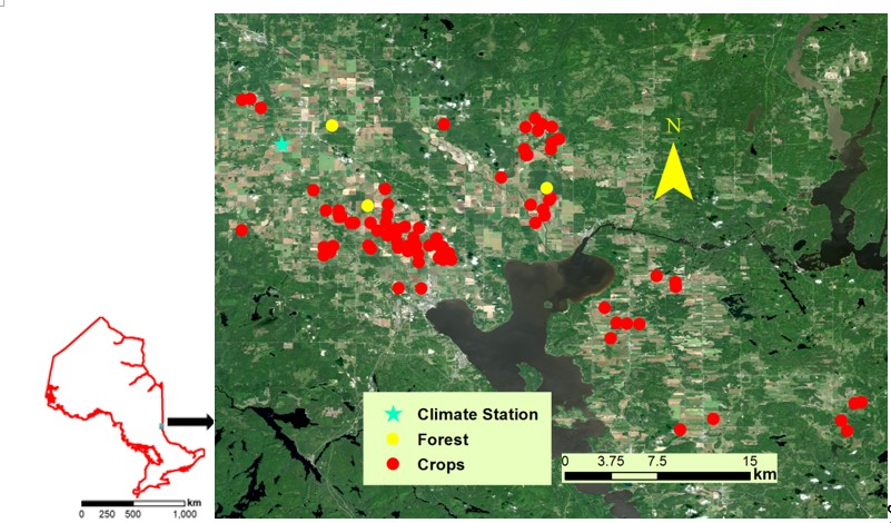
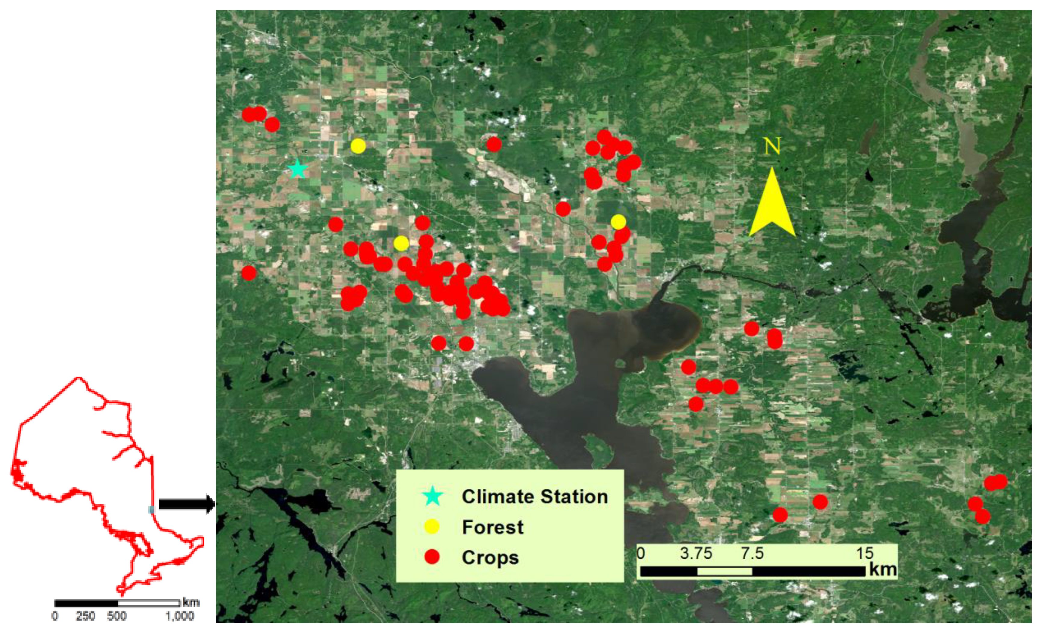
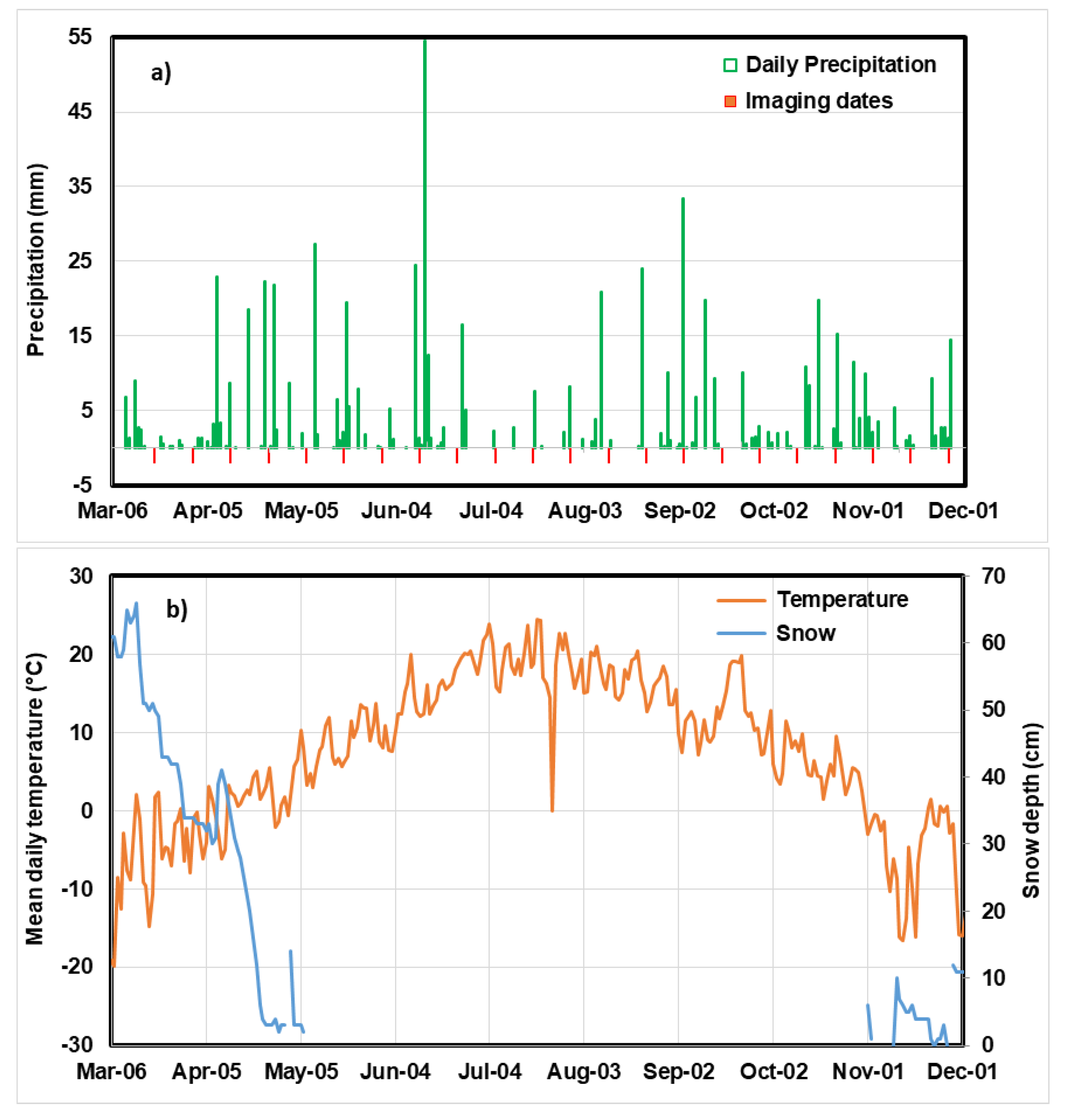
2.1. The Study Site and Field Data

The study is conducted over an agricultural area in Temiskaming Shores, Ontario, Canada (Figure 1). It resides in the Clay Belt at the border between northeastern Ontario and northwestern Quebec. Despite of the long snowy winter and unpredictable rainfalls in a relatively short growing season, the fertile clay soil, climate warming, transportation services and inexpensive lands, have promoted the expansion of agriculture in the region [41]. Major crops include oats, barley, soybean, mixed grain, corn, canola, and hay. Field data were collected from both landowner interviews and planter/harvester recording in the 2019 growing season, which include crop types, and 67 fields for seeding dates and 77 fields for harvest dates (

Table 1. Number of fields observed for 2019 growing season (n = 84).

Crop	Oats	Barley	Canola	Soybean	Spring Wheat	Peas	Total
Seeding	19	9	3	9	20	7	67
Harvest	23	12	5	8	22	7	77

). Spatial distribution of the fields is illustrated in Figure 1. In addition to the crop fields, three forest areas were also identified for comparing their SAR signatures with that of the annual-crop fields. Seasonal meteorological data were also obtained from the Earlton Climate Station maintained by Environment and Climate Change Canada (ID = 6072230). Figure 2 shows daily precipitation (mm), daily mean air temperature (°C), and snow depth on the ground (cm).

2.2. SAR Data and Processing

Interferometric SAR data in SLC (single look complex) format was acquired by the C-band Sentinel-1, the two-satellite SAR constellation system, using the interferometric wide (IW) mode with dual polarizations (VV and VH), for every 12 days. The imagery has a swath of 250-km and spatial resolution of 5 × 20 m. Except for March 7, all images between February 23 and December 8 during the 2019 growing season were acquired, resulting in a total of 24 images. Image acquisition dates are also marked in Figure 2a.

InSAR processing includes the following steps:

• One scene was selected as a master and the terrain observation with progressive scans SAR (TopSAR) bursts relative time information was extracted. The study region was covered by seven bursts from the IW2 sub-swath.
• For each scene in the data stack, the times of the seven master bursts were used to detect the corresponding bursts in each slave scene.
• The data corresponding to the master bursts was extracted in complex format from each ESA data file into the TopSAR data format.
• The master scene was co-registered to a 30 m SRTM (Shuttle Radar Topography Mission) Digital Elevation Model (DEM).
• A first co-registration using amplitude correlation was applied between the master and each of the slave scenes.
• Each co-registered slave scene was re-projected/distorted into the slant-range space of the master scene using the DEM in order to increase the spatial similarities between the scenes.
• A second co-registration between the master and each of the re-projected slave scenes, using both amplitude and interferometric phase, was conducted iteratively until the spatial error falls below 0.001 pixels, required to eliminate phase bias induced by the Doppler effects.
• The co-registered bursts with the phase ramps removed were mosaicked into standard SLC format.
• Interferograms and coherence were created using a 3 × 3 pixels window for coherence estimation. The pixel slant-range sampling corresponds to one look (2.33 m in slant range and 13.4 m in azimuth), with a total spatial sampling of 7 m in slant range and 40 m in azimuth, equivalent to a ground sampling of 12 × 40 m.
• Common band filtering and spatial phase filtering to minimize phase noise and increase interferometric coherence were applied.
• Orthorectification and geocoding to desired projection, i.e., UTM (Universal Transverse Mercator)-17N.

The repeat-pass InSAR processing was conducted for each pair of the temporally consecutive SAR images along the whole growth season. Through the processing, time-series InSAR coherence and SAR backscattering coefficients at VV and VH polarizations were generated. InSAR processing and a sigma-nought calibration were conducted using the Gamma software.

2.3. Data Extraction and Analysis

To study the potential of C-band InSAR data for monitoring crop growth and detecting crop field operations (e.g., seeding or harvest), SAR data, including averages of the backscattering coefficient in VV and VH polarizations, and the VV interferometric coherence, were extracted at the field level within polygons of field boundaries from all SAR acquisitions throughout the season. To prevent interference from headland and different land cover or crop type of neighbouring fields, the polygons were shrunk inward by 50 m using the ArcGIS system software (Esri, CA, USA). It is assumed that the fields were under uniform management condition at any time of SAR image acquisition, although occasionally this may not be true. A dataset consisting of time-series field-level SAR data was then established for visual interpretation and algorithm development to determine the dates of field activities such as seeding and harvest.

3. Results

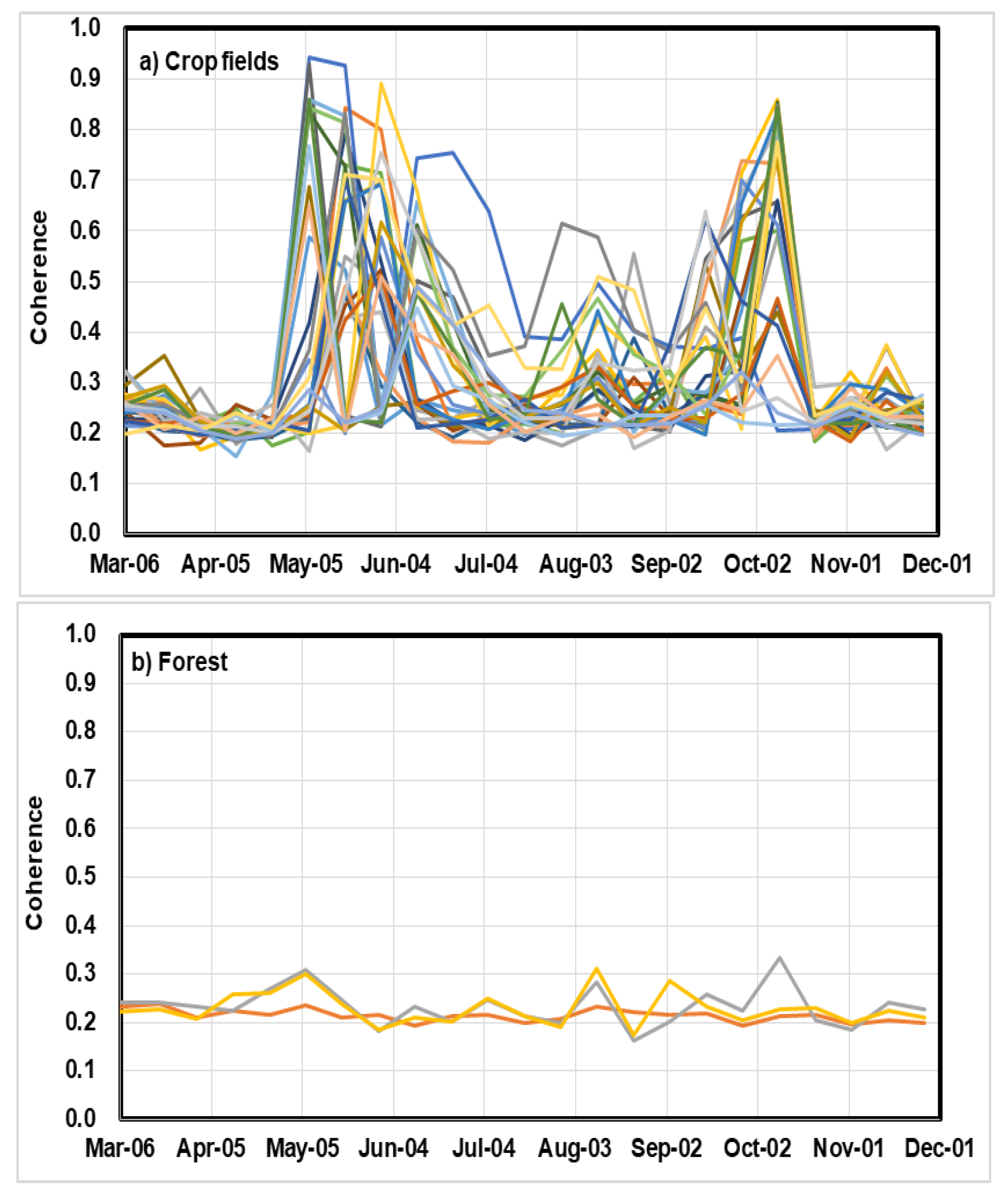
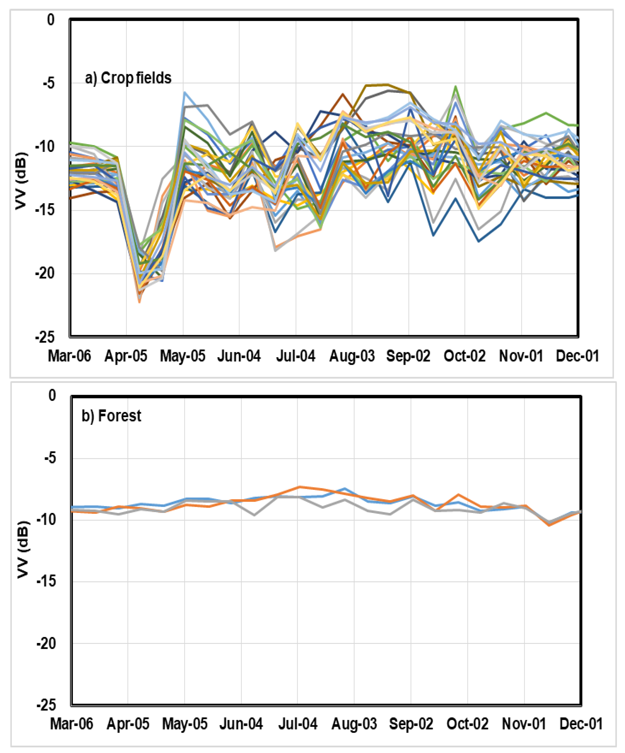
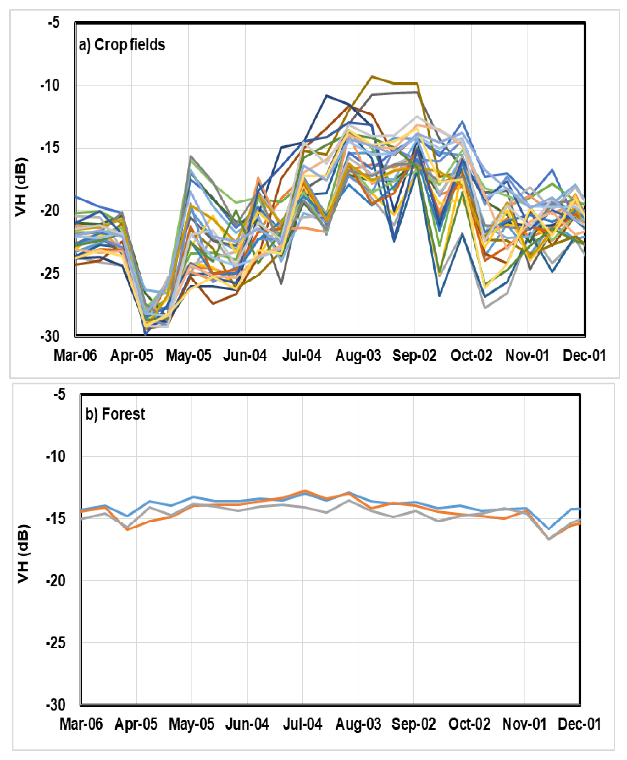
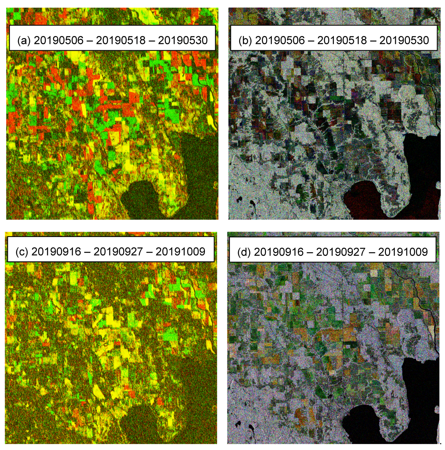
3.1. Seasonal Variation Patterns of InSAR Coherence and SAR Backscattering Coefficient

Seasonal variation of InSAR coherence, SAR backscattering coefficient in VV and VH polarizations are shown in Figure 3, Figure 4 and Figure 5 respectively, for all the observed crop fields and the three patches of forest. For convenience, the dates of the coherence data in Figure 3 represent the acquisition date of the earlier SAR image in each InSAR image pair. It is observed that coherence for the three forest patches remained at a low level (~0.2) throughout the season, whereas that of crop fields showed a wide dynamic range with clear seasonal patterns. The coherence of crop fields was low (0.2–0.3) in the early (before May) and the late (after late October) season. It was at a higher level during the start (May–June) and the end of the growing season (September–October), with a relatively higher coherence at the start of the season than at the end of the season. Coherence generally dropped to a lower level in the mid-season.

The VV and VH backscattering coefficients of the crop fields also exhibited apparent seasonal patterns, with a relatively lower level at the start and the end of the growing season, and a higher level in the middle of the season (August). This trend was more apparent for VH than for VV polarization, and was in accordance with the general seasonal growth cycle of the crops. Large fluctuations throughout the season and great variability among fields were also observed, more for the VV polarization than for VH polarization. For the forest patches, the variation of VV and VH was relatively small throughout the season, with an average of −8.5 dB and dynamic range <3.2 dB for VV, and average −14.3 dB and dynamic range <3.9 dB for VH. VV and VH for the forest were higher than that of the crop fields at the start and the end of the growing season. In April, the backscattering of crop fields was remarkably lower than the rest of the time and that of forest, apparently due to wet snow during spring snow melt.

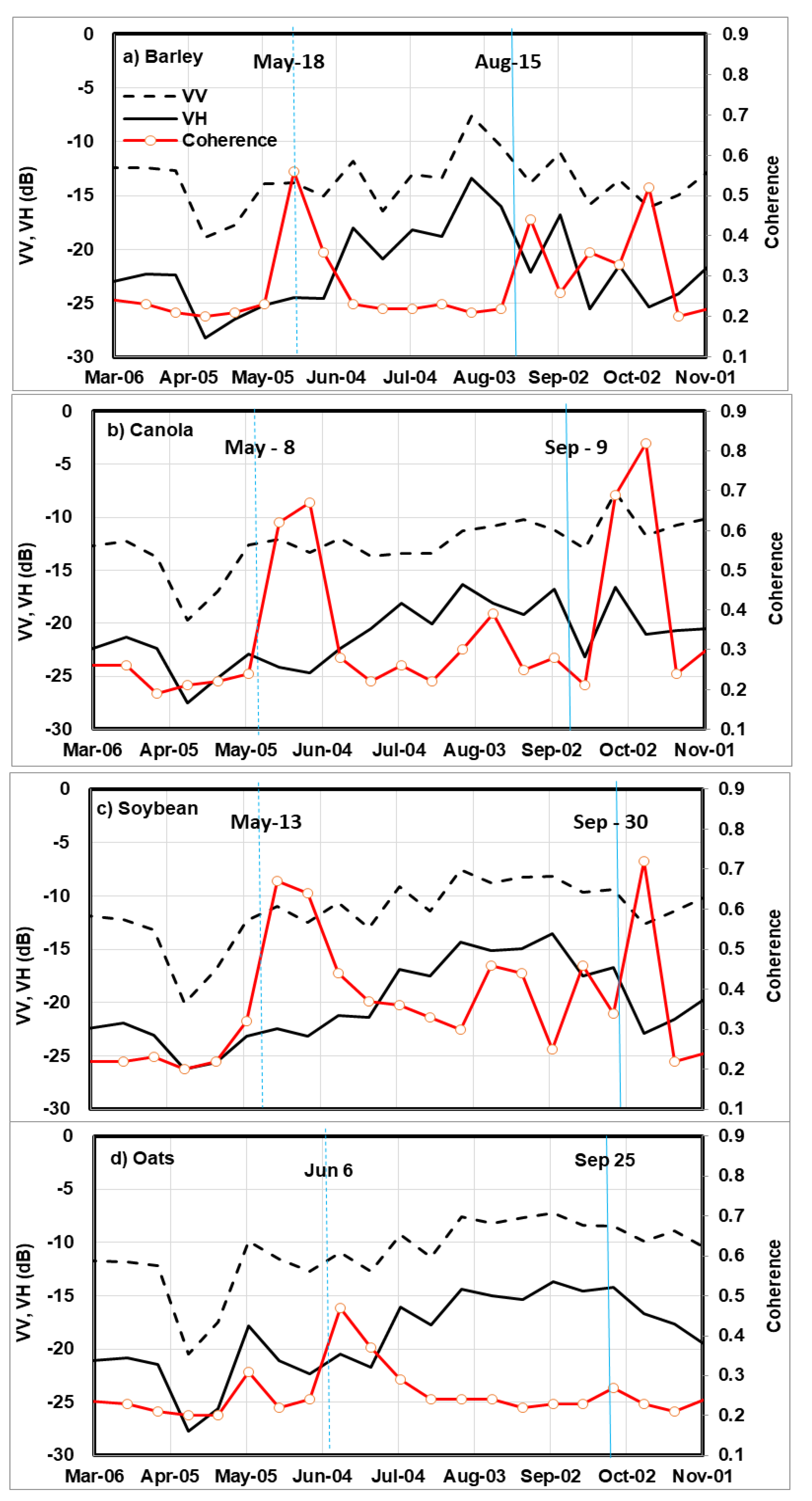
3.2. Relationships between Time-Series SAR Signatures and the Timing of Field Activities

The focus of this study was to estimate crop seeding and harvest dates through change detection based on the analysis of time-series InSAR data. This is built on an assumption that surface roughness or structural conditions of crop fields can be altered by seeding or harvest operations and captured by time-series SAR backscattering and InSAR coherence. However, SAR signals are also affected by other factors, such as soil moisture, precipitation, canopy structural changes associated with plant growth, as well as radar acquisition geometry, although not an issue for Sentinel-1 since by design the interferometric acquisition geometry is kept constant. When interpreting time-series SAR data for crop seeding and harvest date estimation, we took the following aspects into consideration:

(1) VV is mainly related to surface roughness (either soil or upper canopy of the plant), thus can be inspected to infer information on tillage types during the seeding or harvest period when contribution from living plant tissues is relatively small.

(2) For C band, VH is mainly responsive to volumetric scattering and is positively related to the amount of plant tissues; therefore, its signal level is low during seeding to early season and during harvest period. VH tends to reach the highest at full vegetative development stage. This is because the VH polarization mainly reflects the interaction of microwave with the interior parts of the canopy (e.g., volume scattering; Tsyganskaya, et al. [42]), although a double bounce component has been observed by Hong and Wdowinski [43] for flooded vegetation.

(3) InSAR coherence reflects the local phase spatial similarity of two SAR images, which was evaluated within a spatial window of 3 × 3 pixels from an interferogram in this study. A high coherence obtained from a pair of SAR images indicates no change during the period between the two acquisition dates, whereas a low coherence indicates a change has occurred. The coherence levels of two consecutive InSAR pairs can be inspected to infer a change due to field operations. If two interferograms are created from three consecutive SAR scenes, the following scenarios could happen:

• high-high: no change;
• high–low: change in second InSAR period;
• low–high: change in first InSAR period;
• low–low: continuous change.

It is noted that low coherence in general is not necessarily indicative of a change at all time since geometric decorrelation can happen for vegetated surface even when there is no temporal change. As examples, Figure 6a–d depicts time-series InSAR data and the observed seeding and harvest dates for barley, canola, soybean and oats fields, and Figure 7 shows the corresponding post-harvest field photos taken on October 9, 25, 10, and 8, respectively. Pre-harvest photos were taken in the barley and oats field only, on September 16 and August 26, respectively. These four crops are selected for illustrations here because they have quite distinct structures during their life cycles. Average VV and VH and InSAR coherence of the three fields exhibit temporal patterns similar to that outlined in Figure 3, Figure 4 and Figure 5. For the four crops, the VH showed a greater difference between the mid-season and the start/end of the season. This variation pattern followed the variation of amount of fresh biomass present in the field during the growing season, i.e., increase at the growing phase and decrease at the senescent phase. The VV showed a greater dynamic range at the early (May–June) and late (October) growth periods than the VH, possibly because it responded more to vertical structures (such as stems that start developing in the spring and drying up in the fall).

Using the aforementioned interpretation rules, the seeding date for the barley field was determined to be between May 6 and 18, because coherence of the pair of SAR images acquired on these two dates was much lower (~0.23) than that of the next image pair (~0.56), acquired between May 18 and 30 (Figure 6a), which indicated that a great change (i.e., seeding) had happened between the first time window. The harvest date for the field was between August 10 and 22 because there was a big increase in coherence from 0.22 for the August 10 and 22 image pair to 0.44 for the August 22 and September 3 image pair, suggesting that the change (harvest) happened in the first time window. This is in conformity with the observed seeding date on May 18 and harvest date August 15, respectively. In accordance to the low coherence for the August 10–22 InSAR pair, the VH dropped greatly during this period. The low-high coherence transition was also observed afterwards, between September 3 and September 15, and between September 27 and October 9. By referring to the field photo (Figure 7a), we speculate that residue removal might have happened during this period. For the canola field, the observed seeding date was within the time window (May 5–18) determined from time-series InSAR coherence, whereas the observed harvest date (September 9) was earlier by one satellite repeating cycle than the window with the largest InSAR coherence increase (September 15–27 from 0.21 to 0.69) (Figure 6b). It is possible that there is inaccuracy in the reported harvest date by the producer. The smaller InSAR coherence increase during the mid-season is not well understood and will require further study with the support of detailed field observations. For the soybean field, the observed seeding date (May 13) was within the SAR image pair May 6–18, whereas the harvest was captured by the third InSAR coherence increase after late July, i.e., the SAR pair September 27–October 9 (Figure 6c). VH could be inspected to preclude the SAR pairs of July 29–August 8 and September 3–15, based on their relatively higher backscattering coefficients. For the oats field (Figure 6d), VH was large on May 6 and decreased to a lower level on May 30, while coherence increased from May 6 to May 18, and dropped to the lowest level on May 30. This suggests that seeding could have happened during the May 30–June 11 time window, in conformity with the observed seeding date on June 6. It is likely that the field either had cover crop or significant amount of standing residue left from the previous season before seeding. The observed harvest date (September 25) was between the September 15 and 27 time windows. Given the small increase of InSAR coherence (0.04) and a relatively higher level of VH (−14.2 dB) and VV (−9.4 dB), harvest could be during this period, but with less confidence in interpretation.

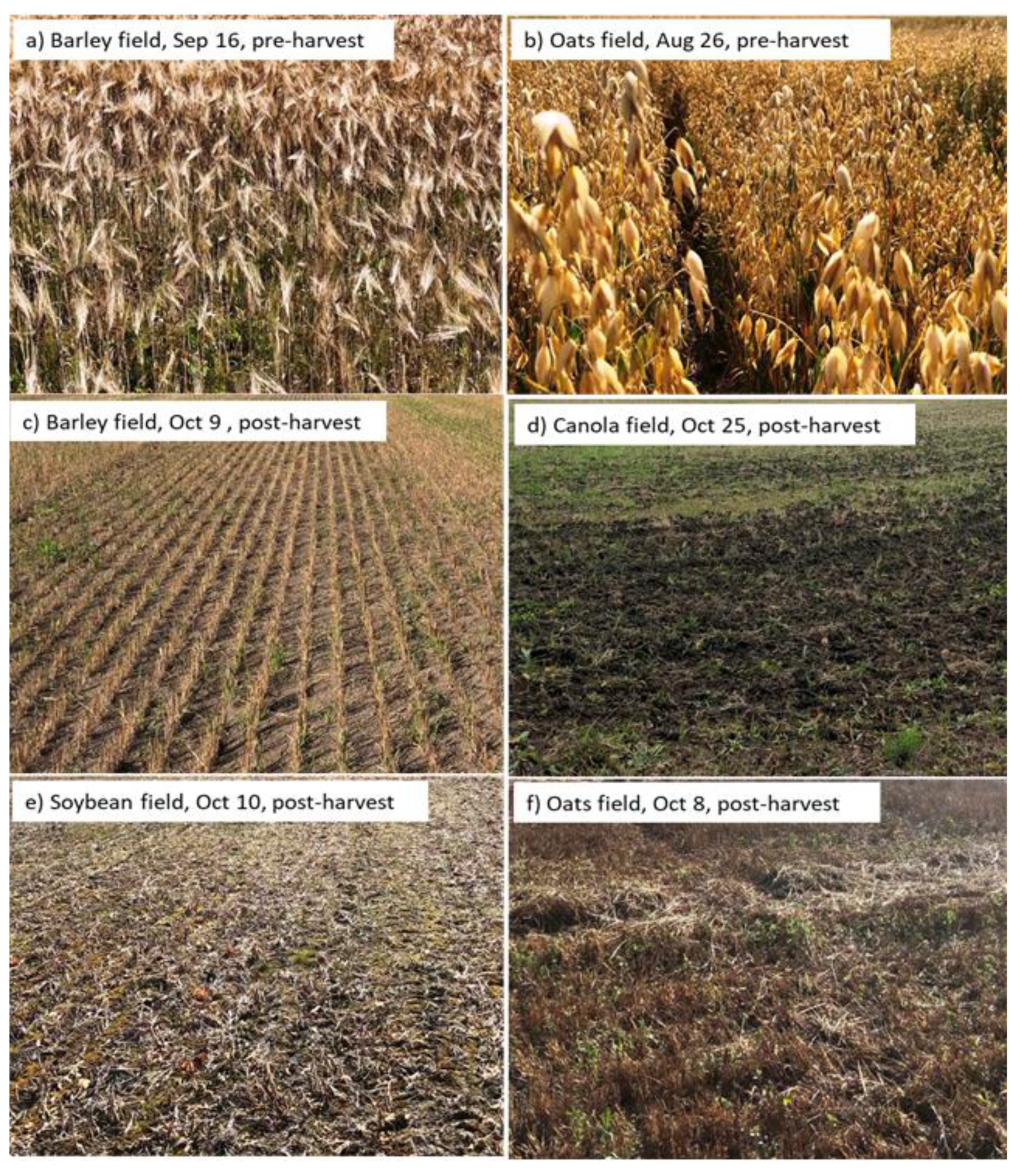
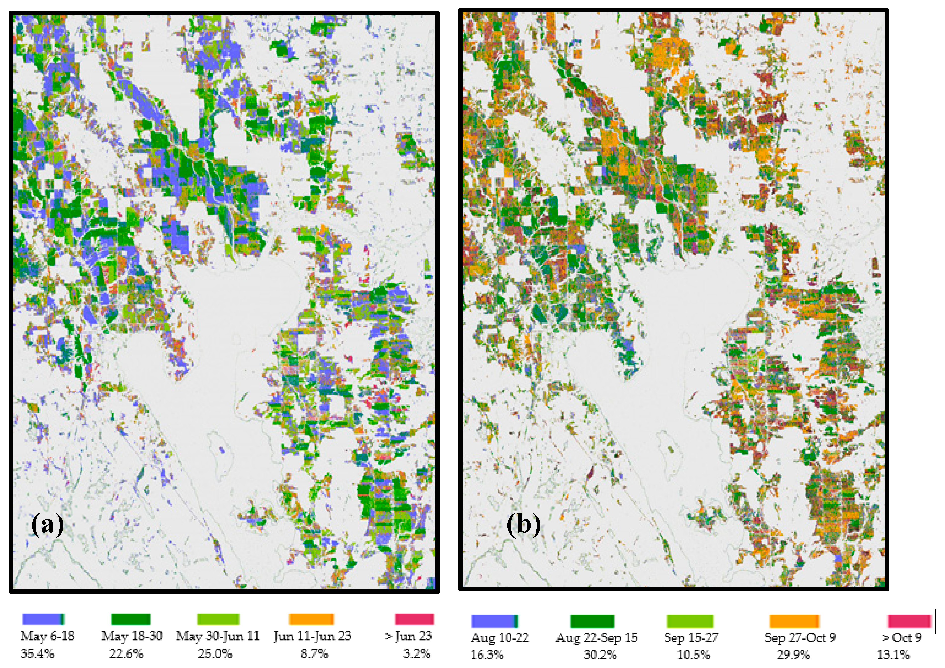
3.3. Determination of Crop Seeding and Harvest Dates

Although detailed field information was not available to allow a more robust and definitive interpretation of the time-series InSAR signatures, yet the examples of these four crop fields showed great promise for using InSAR data to determine the dates of crop seeding and harvest. Two scenarios have been given in previous section to detect the occurrence of change in a field using InSAR coherence, i.e., transition of coherence level from high to low or vice versa. The second scenario is more proper for this study because a relative high coherence is anticipated to last during a period of time after crop seeding but before significant plant development and after harvest when crop fields become more coherent. The following algorithm was thus developed:

(1) Find all candidate InSAR pairs from the beginning to the end of the season, each with an increase of coherence larger than a given threshold value δ° = 0.05.

(2) Determine the time period for seeding activity, with the first candidate date set starting from May 1 to mid-July.

(3) Determine the time period for the harvest activity, with the first candidate date starting from August 1 to end of October.

The threshold of 0.05 was determined based on inspecting the time-series InSAR coherence of example fields. The searching windows for seeding and harvest activities were determined based on local knowledge of general crop phenology in the study region. The period of spring snowmelt (in April) could cause false alarm of seeding activity, thus was excluded from the searching window as seeding can only take place after snowmelt. Due to the more complex situation associated with harvest operation, an additional compound condition was added using VH:

(3a) If VH decreases by more than 2 dB during the same period, or less than 2 dB and is lower than −19 dB at the end of the period, then accept the candidate; otherwise switch to the next candidate and evaluate this additional condition again.

Results using the above algorithm at the field level are reported in

Table 2. Results for seeding and harvest detection.

	Correct	$\pm$1 Cycle	Fail	Total	%Correct
Seeding	57	4	6	67	85
Harvest	43	25	9	77	56

. The accuracy for correct detection of seeding date was 85% (n = 67) and 56% for harvest date (n = 77). For some fields, the observed seeding or harvest dates differed from the detected dates by one satellite acquisition cycle (12 days, the “$\pm$1 Cycle” column on Table 2). This could possibly be related to the fact that field operations such as seeding could sometimes last for several days or longer for a single field. In the case of harvesting, it can even span more than 10 days to complete a field due to various constraints. When these fields are counted, the detection rate increases to 91% for seeding and 88% for harvest. In total, this study failed to detect six fields for seeding and nine fields for harvest, either because no valid change was detected or the detected date was different from the observed date by more than one satellite acquisition cycle.

3.4. Assessment of Time-Series SAR Data for Seeding and Harvest Date Mapping

To illustrate the change due to field operations, colour images were generated and shown in Figure 8 for the period at the beginning of the season in May (May 6 and 18, May 18 and 30) and at the end of the growing season in late September to early October (September 15 and 27, and September 27 and October 9). The images to the left-hand side are made of two InSAR coherence images as the red and green channel, and a blank image (no variance) as the blue channel. The images to the right-hand side are made of the three VH backscattering coefficient as red, green and blue channel. From the images on the left, a field with red color is most likely representing no change during the first pair of SAR acquisition period (hence high coherence) and a change during the second pair of SAR acquisition period (low coherence), whereas green colour likely means that change happened during the first period but no change in the second period. Yellow colour means that coherence is consistently strong and that no structural change happened during both periods. Progression of seeding and harvest in a region can thus be visually evaluated this way through sequential color composition of InSAR coherence images. Images composited with the VH (Figure 8b,d) do not show contrast colour for the changes, but they do highlight the difference between agricultural fields and forests, particularly for the spring image in which crop fields are shown with dark tone, reflecting low biomass or low surface roughness conditions of crop fields in contrast to forests.

To further demonstrate the capability of time-series InSAR coherence and VH backscattering coefficient for identification of crop seeding and harvest dates, the aforementioned algorithm was applied to the SAR data to map crop seeding date at the pixel level. First, crop pixels were identified using a simple threshold approach, i.e., average VH in April < −25 dB and average VH on July 29 and August 10 >−21 dB. This step can effectively exclude the forest (higher VH in April) and water (lower VH in mid-season) pixels in subsequent analysis. Residual speckle noise has caused certain degree of false identification shown as crop pixels on non-agricultural lands. The mapping results are shown in Figure 9 covering five periods for both seeding (Figure 8a,b) and harvest (Figure 8c,d) dates, determined by SAR acquisition dates. The proportion of pixels being identified as seeded or harvested during each time period is also given in Figure 9.

In the study area, crops were seeded mostly in May to early June, with only about 10% of the fields seeded later than June 11. For harvest event, about 16% happened during the period from August 10 to 22, mostly wheat and some other summer cereal crops. For harvest, about 30.2% of the fields were harvest between the two satellite acquisitions from August 22 to September 15. Due to heavy rain at the time of the satellite overpass on September 3, the SAR image was contaminated and hence not used in the analysis. Another 30% of harvest happened between September 27 and October 9, and the rest of the 13% were harvest after October 9.

4. Discussion

Detection of changes due to field operations using InSAR coherence is challenging because a decreased coherence can also be the result of temporal decorrelation caused by natural events, including rain, snow, wind, seasonal changes in vegetation development, and also geometrical decorrelation (from tall and dense vegetation such as forests) [44,45,46]. In this study, we determine crop seeding and harvest through the detection of a sharp change in InSAR coherence, assuming that surface structure will remain stable for a period of time after these two types of field operations, inducing a low coherence for the pair of SAR images spanning the period within which the event happened. However, this cannot always be successful under at least two cases: 1) no-till seeding, for which high coherence could be anticipated because soil surface is not subject to significant interference by the operation, and 2) harvest with substantial amount of residue left standing in the field; in which case, there is low coherence even after harvest. The situation could be further complicated if different management practices are involved after crop harvest: 1) soil tillage at different time with different machine types that can induce different levels of surface roughness; 2) different treatments of crop residues, e.g., residue left standing, chopped and spread, or removed for other purposes at different rates; 3) incorporation of cover crops in the cropping system for soil protection. It was noted in the study area that cover crops developed to a substantial level in some of the summer crop fields after harvest. This reality, although providing challenges in detecting seeding and harvest dates through CCD, also presents an opportunity for the detection of other field operations and crop management practices, such as ploughing.

High coherence can be observed during the mid-season for crops, which may induce ambiguity for the determination of seeding and harvest dates. For instance, the soybean field shown in Figure 6c and has a relatively high coherence (~0.5) in mid-August although the high VH indicated large volume scattering from plant canopy. This may be linked to certain canopy structure characteristics and deserves further investigation. This also illustrates the added value of SAR backscattering to the interpretation of crop field activities. In fact, combination of VV and VH has also been found to be useful for crop type discrimination and biophysical parameter estimation [47,48,49]. This issue could be alleviated with a shorter revisiting cycle of InSAR acquisition because field disturbances can be better resolved in time.

Physical environment conditions, such as snow and rain, can influence not only SAR backscattering signatures but also InSAR coherence [50,51,52]. Low coherence at the beginning and end of season was observed when snow cover was present on the ground and the thaw or freezing process started. According to meteorological records of the nearby station (Figure 2b), snow cover ended at the end of April and started in early November in 2019, thus soil surface (or plant) conditions during these periods will not be captured by the time series SAR data, and SAR data contributed less to interpretation of crop field operations. Although acquisition of radar data is less impacted by weather condition than that of optical sensors, meteorological events can still introduce changes to a certain degree, either in structure or in dielectric property, that are not due to field operations or crop growth dynamics. This can be observed from perturbation of VV and VH intensities during the days reported with precipitation in the later growing season. As shown in Figure 4 and Figure 5, there was an upward spike on September 3 and 27 (Figure 4 and Figure 5), with reported daily precipitation of 33.4 mm and 2.9 mm, respectively (Figure 2). Thus, change detection through time-series SAR data analysis should take into consideration climate conditions at the time of SAR image acquisition.

In this study, a simple algorithm has been developed for the detection the timing of crop seeding and harvest through analysis of time-series InSAR coherence and SAR backscattering coefficients. It is noted that a sigma-nought calibration has been applied on SAR backscattering to ensure signal consistency across space and over time. This is suitable for our study area because of the following reasons: (1) the agricultural land is relatively flat so that variability of SAR signal due to within-field variability of micro-topography or soil variability is small compared with that due to surface structural changes induced by agricultural management practices; (2) with the InSAR acquisition configuration of Sentinel-1, the incidence angle for a given ground area is relatively constant over time, so that angular effects is minimized; (3) the method proposed in this study mainly relies on exploitation of field-level temporal signatures of the time-series SAR backscattering and InSAR coherence. Nevertheless, converting SAR signals to backscattering coefficients as a normalization measure is preferred in most applications. In this study, only 77 fields were surveyed for harvest and 66 of them were recorded with seeding dates. Although the sampling sites were limited for a robust statistical modeling, it is sufficient for analysis based on physical principles, as shown by interpretations of the time-series signatures. An automated procedure could be developed based on the simple rules presented in Section 3.2, however more systematic field observations are needed in order to capture not only seeding and harvest events, but also other events such as pre-planting seedbed preparation, post-harvest residue removal, and fall tillage. The transition between seeding/harvest operations and different field conditions due to other treatments will be different. A larger number of samples will be needed to characterize the signatures of different combinations of field treatments, crop types, and seeding/harvest in order to develop a more robust procedure for automated information extraction.

SAR backscattering coefficients have been exploited intensively for soil and crop parameter retrieval in the literature. Time-series SAR data and InSAR coherence will bring in new dimensions of information for agricultural studies, particularly in detecting but not limited to changes associated with field operations. With two satellites, the Sentinel-1 constellation can acquire data with interferometric capacity at a six-day revisiting cycle. It is anticipated that the Canadian tri-satellite RADARSAT Constellation Mission at four-day repeat time can provide improved capability for agricultural studies.

5. Conclusions

This study investigated the potential of time-series C-band synthetic aperture radar (SAR) data acquired by the Sentinel-1 constellation with interferometric wide mode for determination of crop seeding and harvest dates. Interferometric SAR (InSAR) processing was conducted for each pair of SAR images acquired consecutively in time throughout the 2019 growing season. Preliminary results show through visual interpretation that time-series SAR backscattering revealed the seasonal development cycle of crop growth, while the change in InSAR coherence levels, either a loss of coherence from a high level or a remarkable gain of coherence from a lower level, was associated with substantial change in surface structure of a crop field induced by agricultural land management activities such as seed-bed preparation in the spring or harvest in the fall. This information can be used to deduce the dates on when these field activities happened. However, the loss of coherence can also be associated with other factors, such as temporal decorrelation due to environmental conditions or vegetation development, thus deriving these field activities through InSAR coherence change detection should be integrated with incoherence change detection through the analysis of time-series SAR backscattering as well. Change detection analysis based on time-series SAR data obtained by Sentine-1 and the RADARSAT Constellation Mission can be a research/operation tool for detecting other crop (such as lodging) and field activities that induce sudden and substantial structural changes.

Given the encouraging results from this study, however, the authors also acknowledge the limitations of the reported research. In subsequent study, detailed field observations and in situ measurements concurrent with Sentinel-1 overpass will be collected throughout the growing season from pre-planting to postharvest to better identify all factors contributing to changes in SAR backscattering and InSAR coherence.

References

1. FAO. Transforming the World Through Food and Agriculture—FAO and the 2030 Agenda for Sustainable Development; Food and Agriculture Organization of the United Nations: Rome, Italy, 2017. [Google Scholar]
2. Xue, X.; Pang, Y.; Landis, A.E. Evaluating agricultural management practices to improve the environmental footprint of corn-derived ethanol. Renew. Energy 2014, 66, 454–460. [Google Scholar] [CrossRef]
3. Lee, E.K.; Zhang, W.-J.; Zhang, X.; Adler, P.R.; Lin, S.; Feingold, B.J.; Khwaja, H.A.; Romeiko, X.X. Projecting life-cycle environmental impacts of corn production in the US Midwest under future climate scenarios using a machine learning approach. Sci. Total Environ. 2020, 714, 136697. [Google Scholar] [CrossRef] [PubMed]
4. Kikuchi, Y.; Kanematsu, Y. Life cycle assessment. In Plant Factory, 2nd ed.; Kozai, T., Niu, G., Takagaki, M., Eds.; Academic Press: Cambridge, MA, USA, 2020; pp. 383–395. [Google Scholar]
5. Dong, T.; Shang, J.; Qian, B.; Liu, J.; Chen, J.M.; Jing, Q.; McConkey, B.; Huffman, T.; Daneshfar, B.; Champagne, C. Field-Scale Crop Seeding Date Estimation from MODIS Data and Growing Degree Days in Manitoba, Canada. Remote Sens. 2019, 11, 1760. [Google Scholar] [CrossRef] [Green Version]
6. Urban, D.; Guan, K.; Jain, M. Estimating sowing dates from satellite data over the US Midwest: A comparison of multiple sensors and metrics. Remote Sens. Environ. 2018, 211, 400–412. [Google Scholar] [CrossRef]
7. Manfron, G.; Delmotte, S.; Busetto, L.; Hossard, L.; Ranghetti, L.; Brivio, P.A.; Boschetti, M. Estimating inter-annual variability in winter wheat sowing dates from satellite time series in Camargue, France. Int. J. Appl. Earth Obs. Geoinf. 2017, 57, 190–201. [Google Scholar] [CrossRef]
8. Gao, F.; Masek, J.; Schwaller, M.; Hall, F. On the blending of the Landsat and MODIS surface reflectance: Predicting daily Landsat surface reflectance. IEEE Trans. Geosci. Remote Sens. 2006, 44, 2207–2218. [Google Scholar]
9. Bégué, A.; Arvor, D.; Bellon, B.; Betbeder, J.; De Abelleyra, D.; PD Ferraz, R.; Lebourgeois, V.; Lelong, C.; Simões, M.; Verón, S.R. Remote sensing and cropping practices: A review. Remote Sens. 2018, 10, 99. [Google Scholar] [CrossRef] [Green Version]
10. Joshi, N.; Baumann, M.; Ehammer, A.; Fensholt, R.; Grogan, K.; Hostert, P.; Jepsen, M.R.; Kuemmerle, T.; Meyfroidt, P.; Mitchard, E.T. A review of the application of optical and radar remote sensing data fusion to land use mapping and monitoring. Remote Sens. 2016, 8, 70. [Google Scholar] [CrossRef] [Green Version]
11. Closson, D.; Milisavljevic, N. InSAR Coherence and Intensity Changes Detection. In Mine Action: The Research Experience of the Royal Military Academy of Belgium; Beumier, C., Closson, D., lacroix, V., Milisavljevic, N., Yvinec, Y., Eds.; IntechOpen: London, UK, 2017. [Google Scholar] [CrossRef] [Green Version]
12. Steele-Dunne, S.C.; McNairn, H.; Monsivais-Huertero, A.; Judge, J.; Liu, P.-W.; Papathanassiou, K. Radar remote sensing of agricultural canopies: A review. IEEE J. Sel. Top. Appl. Earth Obs. Remote Sens. 2017, 10, 2249–2273. [Google Scholar] [CrossRef] [Green Version]
13. McNairn, H.; Brisco, B. The application of C-band polarimetric SAR for agriculture: A review. Can. J. Remote Sens. 2004, 30, 525–542. [Google Scholar] [CrossRef]
14. Canisius, F.; Shang, J.; Liu, J.; Huang, X.; Ma, B.; Jiao, X.; Geng, X.; Kovacs, J.M.; Walters, D. Tracking crop phenological development using multi-temporal polarimetric Radarsat-2 data. Remote Sens. Environ. 2018, 210, 508–518. [Google Scholar] [CrossRef]
15. McNairn, H.; Jiao, X.; Pacheco, A.; Sinha, A.; Tan, W.; Li, Y. Estimating canola phenology using synthetic aperture radar. Remote Sens. Environ. 2018, 219, 196–205. [Google Scholar] [CrossRef]
16. Wang, H.; Magagi, R.; Goïta, K.; Trudel, M.; McNairn, H.; Powers, J. Crop phenology retrieval via polarimetric SAR decomposition and Random Forest algorithm. Remote Sens. Environ. 2019, 231, 111234. [Google Scholar] [CrossRef]
17. Fisette, T.; Rollin, P.; Aly, Z.; Campbell, L.; Daneshfar, B.; Filyer, P.; Smith, A.; Davidson, A.; Shang, J.; Jarvis, I. AAFC annual crop inventory. In Proceedings of the 2013 Second International Conference on Agro-Geoinformatics (Agro-Geoinformatics), Fairfax, UA, USA, 12–16 August 2013; pp. 270–274. [Google Scholar]
18. Davidson, A.; Fisette, T.; McNairn, H.; Daneshfar, B.; Delince, J. Detailed crop mapping using remote sensing data (Crop Data Layers). In Handbook on Remote Sensing for Agricultural Statistics; Delince, J., Ed.; The Global Strategy to improve agricultural and rural statistics (GSARS): Rome, Italy, 2017; pp. 91–117. [Google Scholar]
19. Wiseman, G.; McNairn, H.; Homayouni, S.; Shang, J. RADARSAT-2 polarimetric SAR response to crop biomass for agricultural production monitoring. IEEE J. Sel. Top. Appl. Earth Obs. Remote Sens. 2014, 7, 4461–4471. [Google Scholar] [CrossRef]
20. Huang, X.; Wang, J.; Shang, J. Simplified adaptive volume scattering model and scattering analysis of crops over agricultural fields using the RADARSAT-2 polarimetric synthetic aperture radar imagery. J. Appl. Remote Sens. 2015, 9, 096026. [Google Scholar] [CrossRef]
21. Conradsen, K.; Nielsen, A.A.; Skriver, H. Determining the points of change in time series of polarimetric SAR data. IEEE Trans. Geosci. Remote Sens. 2016, 54, 3007–3024. [Google Scholar] [CrossRef] [Green Version]
22. Bouaraba, A.; Belhadj-Aissa, A.; Closson, D. Drastic Improvement of Change Detection Results with Multilook Complex SAR Images Approach. Prog. Electromagn. Res. 2018, 82, 55–66. [Google Scholar] [CrossRef] [Green Version]
23. Osmanoğlu, B.; Sunar, F.; Wdowinski, S.; Cabral-Cano, E. Time series analysis of InSAR data: Methods and trends. ISPRS J. Photogramm. Remote Sens. 2016, 115, 90–102. [Google Scholar] [CrossRef]
24. Ferretti, A.; Monti-Guarnieri, A.; Prati, C.; Rocca, F.; Massonet, D. Guidelines for SAR Interferometry Processing and Interpretation, TM-19, 1st ed.; InSAR Principles; ESA: Noordwijk, The Netherlands, 2007. [Google Scholar]
25. Xue, F.; Lv, X.; Dou, F.; Yun, Y. A Review of Time-Series Interferometric SAR Techniques: A Tutorial for Surface Deformation Analysis. IEEE Geosci. Remote Sens. Mag. 2020, 8, 22–42. [Google Scholar] [CrossRef]
26. Yonezawa, C.; Takeuchi, S. Decorrelation of SAR data by urban damages caused by the 1995 Hyogoken-nanbu earthquake. Int. J. Remote Sens. 2001, 22, 1585–1600. [Google Scholar] [CrossRef]
27. Grey, W.; Luckman, A.; Holland, D. Mapping urban change in the UK using satellite radar interferometry. Remote Sens. Environ. 2003, 87, 16–22. [Google Scholar] [CrossRef]
28. Jung, J.; Yun, S.-H. Evaluation of Coherent and Incoherent Landslide Detection Methods Based on Synthetic Aperture Radar for Rapid Response: A Case Study for the 2018 Hokkaido Landslides. Remote Sens. 2020, 12, 265. [Google Scholar] [CrossRef] [Green Version]
29. Ferretti, A.; Prati, C.; Rocca, F. Permanent scatterers in SAR interferometry. IEEE Trans. Geosci. Remote Sens. 2001, 39, 8–20. [Google Scholar] [CrossRef]
30. Cigna, F.; Bateson, L.B.; Jordan, C.J.; Dashwood, C. Simulating SAR geometric distortions and predicting Persistent Scatterer densities for ERS-1/2 and ENVISAT C-band SAR and InSAR applications: Nationwide feasibility assessment to monitor the landmass of Great Britain with SAR imagery. Remote Sens. Environ. 2014, 152, 441–466. [Google Scholar] [CrossRef] [Green Version]
31. Pepe, A.; Calò, F. A review of interferometric synthetic aperture RADAR (InSAR) multi-track approaches for the retrieval of Earth’s surface displacements. Appl. Sci. 2017, 7, 1264. [Google Scholar] [CrossRef] [Green Version]
32. Even, M.; Schulz, K. InSAR deformation analysis with distributed scatterers: A review complemented by new advances. Remote Sens. Environ. 2018, 10, 744. [Google Scholar] [CrossRef] [Green Version]
33. Torres, R.; Snoeij, P.; Geudtner, D.; Bibby, D.; Davidson, M.; Attema, E.; Potin, P.; Rommen, B.; Floury, N.; Brown, M. GMES Sentinel-1 mission. Remote Sens. Environ. 2012, 120, 9–24. [Google Scholar] [CrossRef]
34. Plank, S. Rapid damage assessment by means of multi-temporal SAR—A comprehensive review and outlook to Sentinel-1. Remote Sens. 2014, 6, 4870–4906. [Google Scholar] [CrossRef] [Green Version]
35. Canisius, F.; Brisco, B.; Murnaghan, K.; Van Der Kooij, M.; Keizer, E. SAR backscatter and InSAR coherence for monitoring wetland extent, flood pulse and vegetation: A study of the Amazon lowland. Remote Sens. 2019, 11, 720. [Google Scholar] [CrossRef] [Green Version]
36. Poncos, V.; Molson, S.; Welch, A.; Brazeau, S. Detection of flooded vegetation and measurements of water level changes using radarsat-2. In Proceedings of the 2013 IEEE International Geoscience and Remote Sensing Symposium-IGARSS, Melbourne, Australia, 21–26 July 2013; pp. 2208–2211. [Google Scholar]
37. Poncos, V.; Molson, S.; Welch, A.; Brazeau, S.; Kotchi, S.O. SAR for surface water monitoring and public health. In Proceedings of the 2014 IEEE Geoscience and Remote Sensing Symposium, Quebec City, QC, Canada, 13–18 July 2014; pp. 1167–1170. [Google Scholar]
38. Khabbazan, S.; Vermunt, P.; Steele-Dunne, S.; Ratering Arntz, L.; Marinetti, C.; van der Valk, D.; Iannini, L.; Molijn, R.; Westerdijk, K.; van der Sande, C. Crop monitoring using Sentinel-1 data: A case study from The Netherlands. Remote Sens. 2019, 11, 1887. [Google Scholar] [CrossRef] [Green Version]
39. Nasrallah, A.; Baghdadi, N.; El Hajj, M.; Darwish, T.; Belhouchette, H.; Faour, G.; Darwich, S.; Mhawej, M. Sentinel-1 Data for Winter Wheat Phenology Monitoring and Mapping. Remote Sens. 2019, 11, 2228. [Google Scholar] [CrossRef] [Green Version]
40. Kavats, O.; Khramov, D.; Sergieieva, K.; Vasyliev, V. Monitoring Harvesting by Time Series of Sentinel-1 SAR Data. Remote Sens. 2019, 11, 2496. [Google Scholar] [CrossRef] [Green Version]
41. Chapagain, T. Farming in Northern Ontario: Untapped potential for the future. Agronomy 2017, 7, 59. [Google Scholar] [CrossRef] [Green Version]
42. Tsyganskaya, V.; Martinis, S.; Marzahn, P.; Ludwig, R. SAR-based detection of flooded vegetation—A review of characteristics and approaches. Int. J. Remote Sens. 2018, 39, 2255–2293. [Google Scholar] [CrossRef]
43. Hong, S.-H.; Wdowinski, S. Double-bounce component in cross-polarimetric SAR from a new scattering target decomposition. IEEE Trans. Geosci. Remote Sens. 2013, 52, 3039–3051. [Google Scholar] [CrossRef]
44. Jung, J.; Kim, D.-j.; Lavalle, M.; Yun, S.-H. Coherent change detection using InSAR temporal decorrelation model: A case study for volcanic ash detection. IEEE Trans. Geosci. Remote Sens. 2016, 54, 5765–5775. [Google Scholar] [CrossRef]
45. Krishnakumar, V.; Monserrat, O.; Crosetto, M.; Crippa, B. Atmospheric phase delay in Sentinel SAR interferometry. In Proceedings of the International Archives of the Photogrammetry, Remote Sensing Spatial Information Sciences, Beijing, China, 30 April 2018; p. 3. [Google Scholar]
46. Olen, S.; Bookhagen, B. Mapping damage-affected areas after natural hazard events using sentinel-1 coherence time series. Remote Sens. 2018, 10, 1272. [Google Scholar] [CrossRef] [Green Version]
47. Veloso, A.; Mermoz, S.; Bouvet, A.; Le Toan, T.; Planells, M.; Dejoux, J.-F.; Ceschia, E. Understanding the temporal behavior of crops using Sentinel-1 and Sentinel-2-like data for agricultural applications. Remote Sens. Environ. 2017, 199, 415–426. [Google Scholar] [CrossRef]
48. Harfenmeister, K.; Spengler, D.; Weltzien, C. Analyzing temporal and spatial characteristics of crop parameters using Sentinel-1 backscatter data. Remote Sens. 2019, 11, 1569. [Google Scholar] [CrossRef] [Green Version]
49. Gherboudj, I.; Magagi, R.; Berg, A.A.; Toth, B. Soil moisture retrieval over agricultural fields from multi-polarized and multi-angular RADARSAT-2 SAR data. Remote Sens. Environ. 2011, 115, 33–43. [Google Scholar] [CrossRef]
50. Li, H.; Wang, Z.; He, G.; Man, W. Estimating Snow Depth and Snow Water Equivalence Using Repeat-Pass Interferometric SAR in the Northern Piedmont Region of the Tianshan Mountains. J. Sens. 2017, 2017, 1–17. [Google Scholar] [CrossRef]
51. Scott, C.; Lohman, R.; Jordan, T. InSAR constraints on soil moisture evolution after the March 2015 extreme precipitation event in Chile. Sci. Rep. 2017, 7, 1–9. [Google Scholar] [CrossRef] [PubMed]
52. Eshqi Molan, Y.; Kim, J.-W.; Lu, Z.; Agram, P. L-band temporal coherence assessment and modeling using amplitude and snow depth over Interior Alaska. Remote Sens. 2018, 10, 150. [Google Scholar] [CrossRef] [Green Version]
Figure 1. Study area in Temiskaming Shores, northern Ontario, overlaid with observed crop fields and forest. Background is a Landsat image acquired on August 24, 2019.
Remotesensing 12 01551 g001
Figure 2. Meteorological condition of the study area in 2019, obtained from the Earlton Climate Station (ID 6072230), Ontario, Canada: (a) daily precipitation; (b) mean daily temperature and snow depth
Remotesensing 12 01551 g002
Figure 3. Typical seasonal variation of InSAR coherence for the study area during May 6–December 1 2019: (a) crop fields and (b) forest.
Remotesensing 12 01551 g003
Figure 4. Typical seasonal variation of VV backscattering coefficients for the study area during May 6–December 1 2019, measured by Sentinel-1 C-band SAR. (a) crop fields and (b) forest.
Remotesensing 12 01551 g004
Figure 5. Typical seasonal variation of VH backscattering coefficients for the study area during May 6–December 1 2019, measured by Sentinel-1 C-band SAR. (a) crop fields and (b) forest.
Remotesensing 12 01551 g005
Figure 6. Time-series SAR data and seeding/harvest dates for example fields of (a) barley, (b) canola, (c) soybean and (d) oats. Vertical blue lines mark the observed seeding date (dashed) and harvest date (solid).
Remotesensing 12 01551 g006
Figure 7. Pre-harvest (a–b) and post-harvest (c–f) photos for the four example fields shown in Error! Reference source not found. Note: no photo was taken in the soybean and canola fields before harvest.
Remotesensing 12 01551 g007
Figure 8. Mapping of change through InSAR coherence at the start May 6–May 18–May 30 (a,b) and end lower, September 15, September 27, and October 9 (c,d) of the season. Maps to the left are generated using two consecutive InSAR coherence images and one blank image as RGB channels (a,c), and maps to the right are made using the three VH backscattering intensity images sequentially as RGB channels (b,d).
Remotesensing 12 01551 g008
Figure 9. Maps of crop seeding (a) and harvest dates (b) derived using time-series InSAR coherence and VH backscattering coefficient. Proportion of pixels identified as seeded or harvested for each time.
Remotesensing 12 01551 g009