Compression of Remotely Sensed Astronomical Image Using Wavelet-Based Compressed Sensing in Deep Space Exploration

1
School of Instrumentation and Optoelectronic Engineering, Beihang University, Beijing 100191, China
2
Key Laboratory of Precision Opto-Mechatronics Technology, Ministry of Education, Beihang University, Beijing 100191, China
*
Author to whom correspondence should be addressed.
Remote Sens. 2021, 13(2), 288; https://0-doi-org.brum.beds.ac.uk/10.3390/rs13020288
Submission received: 12 December 2020
/
Revised: 10 January 2021
/
Accepted: 13 January 2021
/
Published: 15 January 2021
(This article belongs to the Special Issue Wavelet Transform for Remote Sensing Image Analysis)
Abstract
:Compression of remotely sensed astronomical images is an essential part of deep space exploration. This study proposes a wavelet-based compressed sensing (CS) algorithm for astronomical image compression in a miniaturized independent optical sensor system, which introduces a new framework for CS in the wavelet domain. The algorithm starts with a traditional 2D discrete wavelet transform (DWT), which provides frequency information of an image. The wavelet coefficients are rearranged in a new structured manner determined by the parent–child relationship between the sub-bands. We design scanning modes based on the direction information of high-frequency sub-bands, and propose an optimized measurement matrix with a double allocation of measurement rate. Through a single measurement matrix, higher measurement rates can be simultaneously allocated to sparse vectors containing more information and coefficients with higher energy in sparse vectors. The double allocation strategy can achieve better image sampling. At the decoding side, orthogonal matching pursuit (OMP) and inverse discrete wavelet transform (IDWT) are used to reconstruct the image. Experimental results on simulated image and remotely sensed astronomical images show that our algorithm can achieve high-quality reconstruction with a low measurement rate.
1. Introduction
Light-small is the development direction of the optical sensor system in deep space exploration [1,2,3]. This requires the system to execute multiple functions on the same hardware platform [2]. In our previous work, we proposed a miniaturized independent optical sensor system that can provide altitude and navigation information for spacecraft based on optical imaging measurement [3]. Those remotely sensed astronomical images are crucially important for future studies of celestial bodies [4]. Therefore, the system has the functions of image compression and transmission.
Remotely sensed astronomical images impose an urgent demand for compression considering the rapid increase of data, the complexity of the deep space environment, and the performance limitations of airborne equipment [5,6,7,8,9]. Remotely sensed images of extraterrestrial celestial bodies, especially planets, have some unusual features. A typical remotely sensed astronomical image is composed of background and a celestial body [10]. We can significantly reduce the amount of data in the background without losing important information such as geometric structure, edges, and surface textures, which are of great significance for navigation accuracy analysis and scientific exploration [11,12,13]. Therefore, we hope that an optical sensor system will compress remotely sensed astronomical images with a low compression ratio (CR) and low computational complexity while preserving as much information as possible.
Remotely sensed astronomical image compression has been widely studied and applied. Lossless compression can accurately preserve image information and ensure maximum fidelity, but it will hardly meet CR requirements for future deep space exploration [14,15,16,17]. Lossy compression is mainly based on discrete wavelet transform (DWT) and its improved method, which can extract important information through multi-level promotion and meet different compression requirements [18,19,20,21].
Donoho proposed the compressed sensing (CS) theory in 2006, suggesting that a sparse enough signal can be recovered from a small number of measurements, far fewer than required by Nyquist–Shannon sampling theory, substantially reducing sampling frequency and cost of data transmission [22,23]. CS is a linear observation with simple coding and low complexity, and much computation is transferred to the decoding side [24,25]. This is especially suitable to compress remotely sensed astronomical images with a large amount of data and high redundancy. At present, the CS method has a certain application in deep space exploration [18,26,27,28,29,30]. CS has two applications for data compression in deep space exploration. First is analog domain compression, such as the single-pixel aerial remote sensing applied by Ma [28]. Second is digital domain compression, such as CS for 2D compress remotely astronomical data, as proposed by Bobin et al. [29] and Ma et al. [30]. Starck et al. [18] introduced CS that is closely related to sparsity in spatial data compression. CS has the potential for high-efficiency compression of compress remotely astronomical images and leads to performance far exceeding that of JPEG2K [29].
We fully utilize the energy distribution of the remotely sensed astronomical images in the frequency domain and propose a wavelet-based CS algorithm that provides an optimal sampling scheme for an optical sensor system in deep space. Our contributions are summarized as follows. According to the parent–child relationship between the sub-bands and the scanning modes of the high-frequency sub-bands, the wavelet coefficients are rearranged to construct a new sparse vector. An optimized measurement matrix with double allocation measurement rates simultaneously allocates a higher measurement weight to sparse vectors with higher texture detailed complexity and coefficients with higher energy in sparse vectors.
2. Preliminaries
2.1. Discrete Wavelet Transform
The wavelet transform is a powerful time-frequency analysis method that was developed to overcome the Fourier transform’s lack of local capability in the time domain. It has the important property of good localization characteristics in time and frequency domains, and it can provide frequency information of each sub-band of a signal. The discrete wavelet transform (DWT) discretizes the scale and translation of the basic wavelet [31,32].
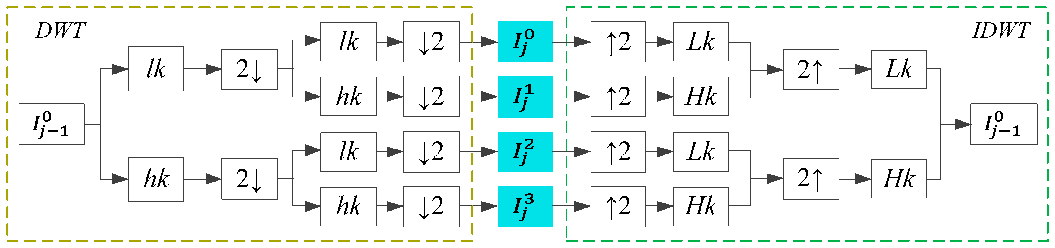
Figure 1 shows the realization of DWT and inverse discrete wavelet transform (IDWT). The image (or low-frequency sub-band of the level) uses low-pass filter and high-pass filter to convolve each raw of the image, and performs downsampling ( indicates column sampling, keeping all even columns). The columns of the image are convolved with and and downsampled ( indicates row sampling, keeping all even rows). Finally, we obtain four sub-images with a size one-fourth of , including: Low-frequency sub-band , horizontal high-frequency sub-band , vertical high-frequency sub-band , and diagonal high-frequency sub-band . The process of reconstruction is opposite that of decomposition. The sub-image is upsampled in the column direction ( means row interpolation, i.e., 0 is filled between adjacent elements), convolved with low-pass filter and high-pass filter , and finally upsampled in the row direction and convolved with and [33]. This step is performed for each layer to obtain the reconstructed image .
The DWT of image is [33]
where is an arbitrary scale, is the size of the image, is the approximate coefficient at scale , and is the scaling function. DWT offers an effective method for 2D matrix transformation from the space domain to the time domain to separate signals according to low and high frequency.
The low-frequency sub-band retains the content information of the original image, and the energy of the image is concentrated in the sub-band. The horizontal and vertical sub-bands maintain the high-frequency information in the horizontal and vertical directions, respectively. The diagonal sub-band maintains high-frequency information in the diagonal direction.
2.2. Compressed Sensing
CS shows [22,23] that if a signal is sparse in a certain transform domain, an observation matrix is used to project the signal linearly. By solving a convex optimization problem, the signal can be recovered [34]. CS effectively solves the limitation of the Nyquist theorem on the sampling rate and the waste of data caused by conventional compression.
This sparse representation of the signal is the basis of CS. Assuming that signal is sparse under the sparse basis , the sparse representation is
where is the length of . The matrix form is
where is the sparse representation of .
is a measurement matrix of size ). Sampling (measurement) is a process of linear projection. The compressed signal is
where is a sensing matrix. It is a problem of an ill-conditioned underdetermined equation. If and satisfy the restricted isometry property (RIP), i.e., for any constant ,
then coefficients (the sparsity of is ) can be accurately reconstructed. The minimum value of is the RIP constant. The equivalent of RIP is that and are orthogonal.
Signal reconstruction is an optimal solution problem of , but it is NP-hard [25]. Therefore, it is often replaced by the optimal solution problem of :
where is the reconstructed signal and is the norm of . Most reconstruction algorithms are iterative greedy, convex optimization, or combination algorithms. Iterative greedy algorithms obtain the sparse vector support set of the source signal, and use the least squares estimation algorithm with limited support to reconstruct the signal [35]. Representative algorithms include matching pursuit [36] and orthogonal matching pursuit (OMP) [37]. Convex optimization algorithms convert a non-convex problem to a convex problem that is solved to approximate the source signal. Representative algorithms include basis pursuit [38] and gradient projection [39]. Combined algorithms have a high reconstruction speed, but they obtain a high probability rather than an accurate reconstruction.
3. Proposed Technique
In deep space exploration, our focus in the image compression of the optical sensor system is the compression (sampling) process. CS uses sparsity to perform linear compression at encoding, and nonlinear reconstruction at decoding. It effectively saves the cost of encoding and transfers the calculation cost to decoding. Therefore, it is highly suitable for remotely sensed astronomical images with a large amount of data and high redundancy in deep space exploration.
The encoding of CS has two main parts: The sparseness and the measurement matrix. The sparseness of DWT is better than that of other sparse bases, but conventional sparse vectors do not define a structure for wavelet coefficients. A method was proposed to average the wavelet coefficient matrix to construct sparse vectors [40]. Such methods do not consider the dependency between sub-bands and the direction information of high-frequency sub-bands, which will lead to poor performance in image compression. However, the fixed and improved measurement matrix cannot optimally allocate the measurement rate, and no measurement matrix is available to consider both sparse vectors and their elements. Therefore, we combine a new structured manner sparse vector and an optimized measurement matrix to design an optimal sampling scheme. The details of our proposed algorithm are as follows.
3.1. A New Sparse Vector Based on the Rearrangement of Wavelet Coefficients
The real signal in nature has sparseness in the transform domain. We can perform compression sampling for the sparse signal. The sparse representation is the essential premise and theoretical basis of CS. In this section, we construct a new sparse vector by rearranging the wavelet coefficients according to the energy distribution of the image after DWT.
For a given remotely sensed astronomical image , the j-level DWT is applied to obtain the transformed image , which has sub-bands. The size of satisfies and , where and are natural numbers. The dimension of the i-level sub-band is . includes the low-frequency sub-band , which reflects the approximate information of the image, and high-frequency sub-bands ,, and , , reflecting the detailed information.
Figure 2a shows the tree structure of the three-level DWT. Low- and high-frequency sub-bands and are at the upper-left and bottom-right corners, respectively. There is a parent–child relationship between sub-bands. The direction of the arrow is from parent to child. Except for , , , and , one parent node corresponds to four child nodes: , , , and . In low-frequency sub-band , each node has only three child nodes: , , and . When , , and are regarded as parent sub-bands, the corresponding child sub-bands are , , and , respectively. Similarly, , , and are child sub-bands of , , and , respectively. High-frequency sub-bands , , and have no child sub-band. The idea of this parent–child relationship is that the parent sub-band node and the corresponding child sub-band nodes reflect the same area information of the image. The parent sub-band has a higher importance than the child sub-band. At the same level of sub-bands, the low-frequency has the highest importance, and the importance of high frequency sub-bands, in descending order, is ,, and [41]. The parent–child relationship is the basis for calculation of the texture detailed complexity and design of the measurement matrix.
We design a data structure to represent sparse vector, , according to the parent–child relationship. Figure 2b shows the first column, of the sparse vector, , and its arrangement order is as follows (j = 3):
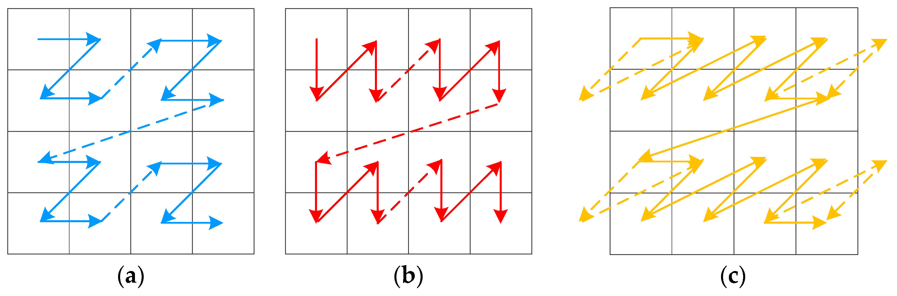
where , , and represent the horizontal, vertical, and diagonal z-scan modes, respectively. For example, represents the diagonal z-scan mode to arrange the coefficients of the block in . When we design a sparse vector, we must specify the block-scanning mode. This is based on the direction information of the high-frequency sub-bands. The horizontal z-scan mode is used for , and reflects horizontal direction information; the vertical z-scan mode is used for , and reflects vertical direction information; sub-band , which reflects diagonal direction information, adopts the diagonal z-scan mode. Conventional CS sampling (measurement) is performed on each column (or each column of the sub-bands) of the coefficient matrix obtained by the DWT of the image [42,43]. High-frequency sub-bands contain the direction information of the image [44]. The performance of CS can be further improved if this characteristic can be used. Therefore, we use different scanning modes for blocks in high-frequency sub-bands. The horizontal, vertical, and diagonal z-scan modes are shown in Figure 3. The solid line in Figure 3c represents the actual scan order.
In the new sparse vector, the number of elements contained in is
where . The new sparse vector is
Table 1 shows the number of sparse vectors and their lengths for different wavelet decomposition levels.
3.2. Measurement Matrix with Double Allocation Strategy
The measurement matrix is used to observe the high-dimensional original signal to obtain the low-dimensional compressed signal. That is, the original signal is projected onto the measurement matrix to obtain the compressed signal. In this section, depending on the parent–child relationship between sub-bands and scanning modes for high-frequency sub-bands, we design a new sparse vector to achieve an optimal measurement rate allocation scheme. The new sparse vector has some unique characteristics. Each sparse vector is composed of a low-frequency sub-band coefficient and multiple high-frequency sub-band coefficients. Elements in the same sparse vector have different importance degrees. The elements of each sparse vector are the frequency information of the same area in the image. The sparse vectors have different importance to image reconstruction; image areas with rich texture are more important.
Therefore, we propose an optimized measurement matrix with a double allocation of measurement rates, which has the advantage that the effects of sparse vectors and their elements on the measurement rate allocation are considered simultaneously. For different sparse vectors, we allocate higher measurement rates to important sparse vectors. In a sparse vector, more weight is given to important elements. The main steps are as follows.
- An random Gaussian matrix is constructed.
- In a sparse vector, the importance of the elements decreases from the front to the back. Increasing the coefficient of the first half of the measurement matrix can preserve more important information of the image. To do this, and to satisfy the incoherence requirement of any two columns of the measurement matrix, we introduce an optimized matrix,where and are different prime numbers. Since and are relatively prime, any two columns of are incoherent [45,46].
- The upper left part of is dot-multiplied with , and other coefficients of remain unchanged, to obtain an optimized measurement matrix . Because and , the coefficients of the upper-left part of are increased.
- is the size of . It is determined by the measurement rate of each sparse vector. When the total measurement rate is certain, the measurement rate is allocated according to the texture detail complexity of the image. We calculate as follows.
- The elements in the sparse vector correspond to the frequency information of the same area in the image. The high-frequency coefficients reflect the detailed information. The energy of high-frequency coefficients is defined to describe the texture detailed complexity of the sparse vector. Taking as an example, the energy of the high-frequency coefficients of iswhere represents the i-th element in .
- If the total measurement rate is , then the total measurement number isis divided into two parts: Adaptive distribution and fixed distribution. The measurement number used to adaptively allocate according to the complexity of the texture isThe measurement number of fixed allocation isi.e., is evenly allocated to each sparse vector.
- The higher the texture detailed complexity, the higher measurement rates are allocated to ensure retention of more details. Image areas with low texture detailed complexity, such as the background and smooth surface areas, are allocated lower measurement rates. The measurement rate is adaptively allocated according to the texture detailed complexity. A linear measurement rate allocation scheme is established based on this principle. The measurement number of the sparse vector iswhere is the number of sparse vectors, andis a proportionality coefficient. Then the measurement number of isand the final measurement number of is , i.e.,
- The sparse vectors are compressed by the optimized measurement matrix, and the compressed value of is
3.3. Image Reconstruction
The reconstruction is an optimal solution problem for solving ,
where is the recovered sparse matrix, is the abbreviation of “subject to”. We use the OMP algorithm to reconstruct sparse vectors [25]. OMP is a classical greedy iterative algorithm that follows the atomic selection strategy of the matching tracking algorithm. Each iteration selects an atom, and the selected atomic set should be normalized in each iteration to ensure the optimization of each iteration result, thus reducing the number of iterations and accelerating convergence. OMP performs vector orthogonalization during each iteration. OMP has higher space and time complexity than the matching pursuits method. In deep space exploration, our optical sensing system compresses remotely sensed astronomical images and transmits the compressed data, and associated calculation costs, to the ground. The recovered vectors are rearranged into a discrete wavelet coefficient matrix, and the reconstructed image is obtained through an inverse discrete wavelet transform.
4. Experimental Results and Analysis
4.1. Evaluation Standard
The peak signal to noise ratio (PSNR) and structural similarity (SSIM) [47] are employed as evaluation indexes of the reconstructed image quality. The PSNR is widely used to measure the distortion effect after compression. As a quantitative measure to the subjective quality, the SSIM demonstrates the quality of detailed information such as the textures and edges of the reconstructed image [48].
The PSNR of an image is
where
is the mean square error, and and , respectively, represent the original and reconstructed image. For a color image,
where stands for the three channels in the image. In this paper, we converted RGB images to YUV channels for processing.
The SSIM evaluates the luminance, contrast, and structure of the image. It can be represented as:
where , , , and are the local mean, variance, and cross-covariance for and .
where is the maximum value of pixel gray, , . For a color image, the SSIM value is the average of the three channels.
4.2. Experimental Data and Evaluation
Experiments were performed on a simulated celestial body image, the gibbous moon, and images of planets, and the experimental results were evaluated subjectively and objectively by comparing three algorithms. Image compression in deep space detection is mainly based on JPEG2K, an algorithm with wavelet transform as the core technology. Starck et al. [29] analyzed the application and advantages of traditional CS algorithms on astronomical images. Traditional CS algorithms compress each column of the sparse matrix after DWT and use a random Gaussian measurement matrix with a fixed measurement rate. A DWT-CS algorithm proposes [40] to construct a sparse vector, giving more weight to higher energy coefficients. Three-level DWT is performed on an image using a coif5 wavelet. The prime numbers and of the measurement matrix are 2 and 3, respectively. The images of moon and planets are taken from Celestial, which is an open-source software for astronomical works supported by NASA Technology [49]. The PSNR and SSIM are the average of 1000 experiments.
4.2.1. Simulated Images of Celestial Bodies
A simulated celestial body image can be obtained by calculating the number of photoelectrons on each illuminated pixel [10]. The number of photoelectrons is
where is the quantum efficiency of the image sensor, is the fill factor, is a single pixel area, is the exposure time, and the total photon flux hitting the pixel is
where is the radiance of the reflected light, is the transmittance of the optics, is the aperture diameter, is the focal length, and is the angle between the line-of-sight vector and the observer surface normal [10].
The celestial body imaging model is the convolution of the cumulative energy distribution of the optical sensor system with the [3],
where is the point spread function of the optical system, and is the convolution operation.
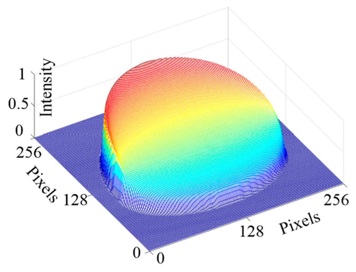
We simulated a 256 × 256 celestial body image whose radius was 100 pixels. Figure 4 displays its normalized intensity distribution model. Table 2 and Table 3, respectively, show the values of PSNR and SSIM when CR is 0.1, 0.2, 0.3, 0.4, 0.5, and 0.6. In this paper, the CR is the ratio of the compressed image to the original image.
When CR is low, the CS, DWT-CS, and the proposed algorithm perform better than JPEG2K because CS takes advantage of sparsity and can restore the original data through a lower sampling rate. As CR increases, the reconstruction quality of JPEG2K improves significantly. JPEG2K achieves low CR and high fidelity with difficulty, resulting in a long transmission time or a poor image quality [50]. The proposed algorithm performs best when CR is 0.1–0.6. It constructs a new sparse vector based on the energy distribution of the image in the frequency domain and the information carried by the sub-bands, and double allocation of the measurement rate can realize an optimal sampling scheme. When the total measurement rate is determined, more measurement weight is given to the sparse vector with richer surface texture and elements with higher energy, ensuring better reconstruction quality at a lower CR.
4.2.2. Moon Image
As the starting point of human deep space exploration, the moon has great significance. Figure 5 shows the moon image and a partial enlargement. The moon has abundant features, such as texture, edges, and lunar mare.
Table 4 compares the PSNR values of the four algorithms. The CR ranges from 0.1 to 0.6, and the interval is 0.1. The PSNR values of the four algorithms increase with CR. Compared to JPEG2K, the PSNRs of the proposed algorithm improve by 7.2812 and 1.9110 dB when CR is 0.1 and 0.6, respectively. The PSNR of the proposed algorithm improves by 2–6 dB compared to CS and DWT-CS.
Table 5 shows the SSIM values of the four algorithms. When CR is 0.1, compared with JPEG2K, CS, and DWT-CS, the SSIM values of the proposed algorithm are improved by 0.1351, 0.0877, and 0.0583, respectively. When CR is 0.1–0.6, the SSIM of the proposed algorithm show the best performance, which indicates that our algorithm can retain more texture information at the same CR compared with other algorithms.
Figure 6 shows part of the reconstructed image when the CR is 0.1 and 0.6. When the CR is low, the reconstructed image of JPEG2K has obvious distortion. With the increase of CR, the quality of the reconstructed images by the four algorithms improves significantly. Comparing the edge and surface textures of the reconstructed image, the proposed algorithm performs better than the others. The scanning mode based on direction information and the measurement rate allocation strategy shows a significantly improved reconstruction effect.
4.2.3. Planet Image
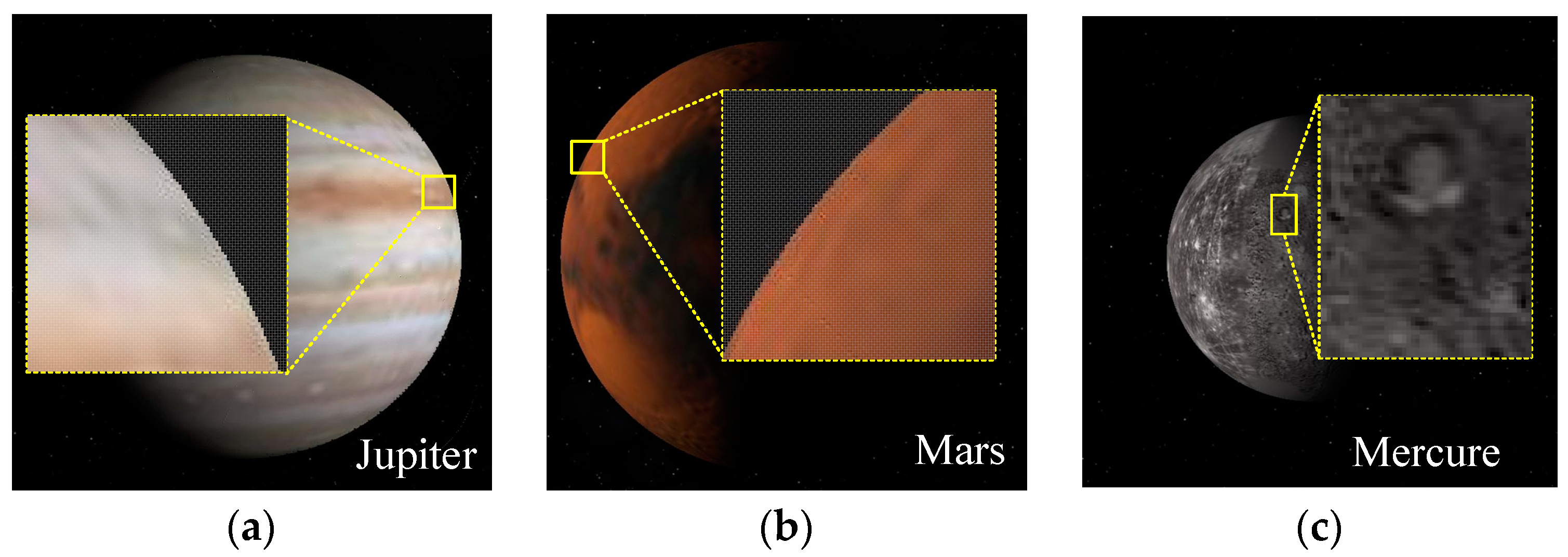
Planets, especially Mars, are new directions for deep space exploration. Figure 7a–c show original and partial enlarged views of Jupiter, Mars, and Mercury, respectively.
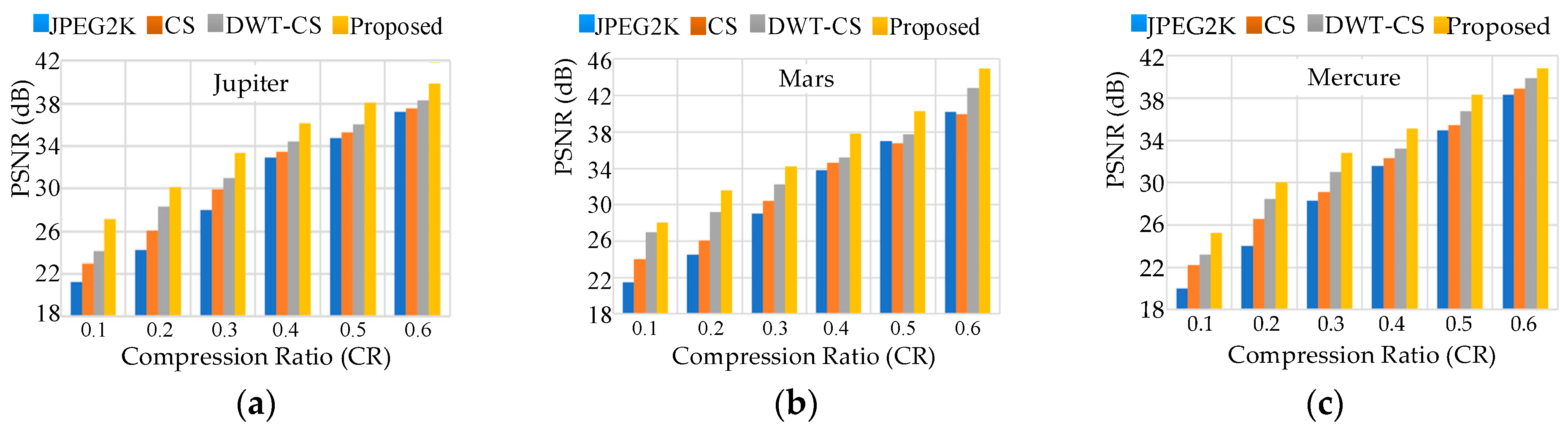
We analyze the average PSNR and SSIM of the three planets. Figure 8 shows the PSNR values of the three planets when CR is 0.1–0.6 (with an interval of 0.1), and all increase with CR. The proposed algorithm has evident advantages when CR is 0.1, with PSNR values increasing by 6.3291, 4.2989, and 2.9640 dB, respectively, compared to JPEG2K, CS, and DWT-CS. The values of the algorithms are relatively close when CR is 0.6, increasing by 2.8765, 2.7942, and 1.6371 dB for the proposed algorithm over JPEG2K, CS, and DWT-CS, respectively. Table 6 shows the SSIM values of the three planets. When CR is 0.1–0.6, compared with the other three algorithms, the SSIM of the proposed algorithm have better performance. When CR is 0.1, compared with JPEG2K, CS, and DWT-CS, the SSIM values of the proposed algorithm are improved by 0.1010, 0.0839, and 0.0521, respectively. When CR is low, the reasonable use of the measurement rate is particularly important. Our double allocation scheme can optimally allocate the limited measurement rate to obtain a better reconstructed image.
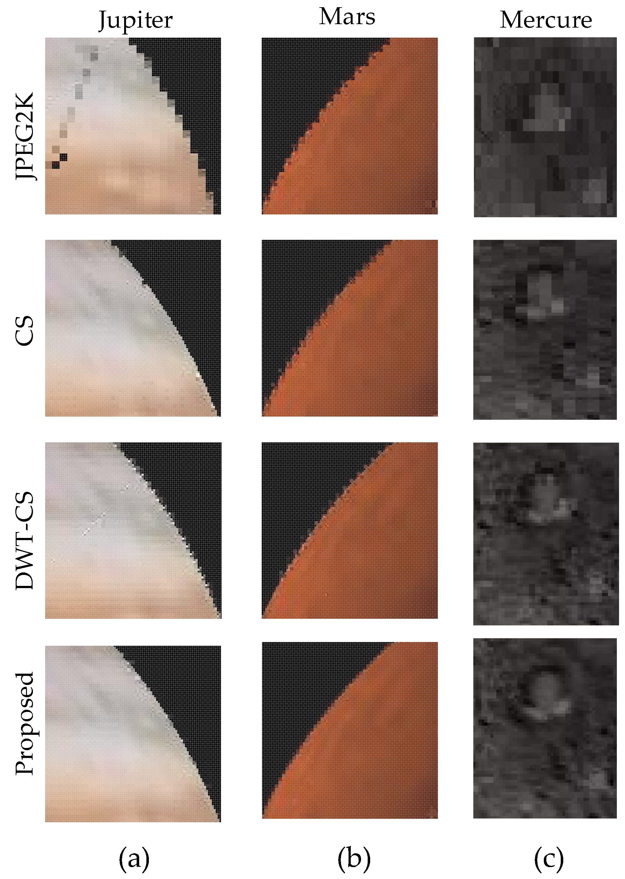
Figure 9 shows a partially enlarged view of the reconstructed images when CR is 0.1. We analyze the edges of Jupiter and Mars. The image edges reconstructed by the four algorithms are all distorted. In particular, for JPEG2K, the edge distortion is more serious, and the blocking effect is evident. Our algorithm also has distortions that can be distinguished, but it performs better than the other algorithms. Impact craters are used to analyze the reconstruction effect of Mercury. Compared to the original image, the other algorithms have obvious distortions, and the reconstruction effect of our algorithm is closest to the original image. Our algorithm preserves the shape of the impact crater and obtains better reconstruction quality.
5. Conclusions
We presented a wavelet-based sensing algorithm to compress remotely sensed astronomical images, fully considering the characteristics of an image in the frequency domain and using a sparse matrix construction method based on the parent–child relationship between sub-bands and different scanning modes of high-frequency sub-bands. The optimized measurement matrix with a double allocation of measurement rates provides an optimal measurement rate allocation strategy. The optimized measurement matrix retains the most important information of the frequency domain at a low measurement rate. An astronomical image was reconstructed by OMP and IDWT. The proposed algorithm was verified on remotely sensed astronomical images. Experiments demonstrated its advantages in PSNR and SSIM compared to JPEG2K, CS, and DWT-CS. We have provided a high-performance remotely sensed astronomical image compression algorithm for a miniaturized independent optical sensor system in deep space exploration. The algorithm has a certain reference significance for other images with a rich texture.
Author Contributions
Y.Z. is responsible for the research ideas, overall work, the experiments, and writing of this paper. J.J. provided guidance and modified the paper. G.Z. is the research group leader who provided general guidance during the research and approved this paper. All authors have read and agreed to the published version of the manuscript.
Funding
This research was supported by the National Natural Science Foundation of China (No. 61725501).
Institutional Review Board Statement
Not applicable.
Informed Consent Statement
Not applicable.
Data Availability Statement
Not applicable.
Acknowledgments
Careful comments given by the anonymous reviewers helped improve the manuscript.
Conflicts of Interest
The authors declare no conflict of interest.
References
- Ma, X.; Fang, J.; Ning, X. An overview of the autonomous navigation for a gravity-assist interplanetary spacecraft. Prog. Aerosp. Sci. 2013, 63, 56–66. [Google Scholar] [CrossRef]
- Jiang, J.; Wang, H.; Zhang, G. High-accuracy synchronous extraction algorithm of star and celestial body features for optical navigation sensor. IEEE Sens. J. 2018, 18, 713–723. [Google Scholar] [CrossRef]
- Zhang, Y.; Jiang, J.; Zhang, G.; Lu, Y. Accurate and Robust Synchronous Extraction Algorithm for Star Centroid and Nearby Celestial Body Edge. IEEE Access 2019, 7, 126742–126752. [Google Scholar] [CrossRef]
- Blanes, I.; Magli, E.; Serra-Sagrista, J. A Tutorial on Image Compression for Optical Space Imaging Systems. IEEE Geosci. Remote Sens. Mag. 2014, 2, 8–26. [Google Scholar] [CrossRef] [Green Version]
- Hernández-Cabronero, M.; Portell, J.; Blanes, I.; Serra-Sagristà, J. High-Performance lossless compression of hyperspectral remote sensing scenes based on spectral decorrelation. Remote Sens. 2020, 12, 2955. [Google Scholar] [CrossRef]
- Magli, E.; Valsesia, D.; Vitulli, R. Onboard payload data compression and processing for spaceborne imaging. Int. J. Remote Sens. 2018, 39, 1951–1952. [Google Scholar] [CrossRef] [Green Version]
- Báscones, D.; González, C.; Mozos, D. An FPGA accelerator for real-time lossy compression of hyperspectral images. Remote Sens. 2020, 12, 2563. [Google Scholar] [CrossRef]
- Rui, Z.; Zhaokui, W.; Yulin, Z. A person-following nanosatellite for in-cabin astronaut assistance: System design and deep-learning-based astronaut visual tracking implementation. Acta Astronaut. 2019, 162, 121–134. [Google Scholar] [CrossRef]
- Orlandić, M.; Fjeldtvedt, J.; Johansen, T. A Parallel FPGA Implementation of the CCSDS-123 Compression Algorithm. Remote Sens. 2019, 11, 673. [Google Scholar] [CrossRef] [Green Version]
- Christian, J.A. Optical Navigation for a Spacecraft in a Planetary System. Ph.D. Thesis, Department of Aerospace Engineering, The University of Texas, Austin, TX, USA, 2010. [Google Scholar]
- Mortari, D.; de Dilectis, F.; Zanetti, R. Position estimation using the image derivative. Aerospace 2015, 2, 435–460. [Google Scholar] [CrossRef] [Green Version]
- Christian, J.A. Optical navigation using planet’s centroid and apparent diameter in image. J. Guid. Control. Dyn. 2015, 38, 192–204. [Google Scholar] [CrossRef]
- Christian, J.A.; Glenn Lightsey, E. An on-board image processing algorithm for a spacecraft optical navigation sensor system. AIAA Sp. Conf. Expo. 2010, 2010. [Google Scholar] [CrossRef]
- Guerra, R.; Barrios, Y.; Díaz, M.; Santos, L.; López, S.; Sarmiento, R. A new algorithm for the on-board compression of hyperspectral images. Remote Sens. 2018, 10, 428. [Google Scholar] [CrossRef] [Green Version]
- Weinberger, M.J.; Seroussi, G.; Sapiro, G. The LOCO-I lossless image compression algorithm: Principles and standardization into JPEG-LS. IEEE Trans. Image Process. 2000, 9, 1309–1324. [Google Scholar] [CrossRef] [PubMed] [Green Version]
- Du, B.; Ye, Z.F. A novel method of lossless compression for 2-D astronomical spectra images. Exp. Astron. 2009, 27, 19–26. [Google Scholar] [CrossRef]
- Aiazzi, B.; Selva, M.; Arienzo, A.; Baronti, S. Influence of the system MTF on the on-board lossless compression of hyperspectral raw data. Remote Sens. 2019, 11, 791. [Google Scholar] [CrossRef] [Green Version]
- Starck, J.L.; Bobin, J. Astronomical data analysis and sparsity: From wavelets to compressed sensing. Proc. IEEE 2010, 98, 1021–1030. [Google Scholar] [CrossRef] [Green Version]
- Pata, P.; Schindler, J. Astronomical context coder for image compression. Exp. Astron. 2015, 39, 495–512. [Google Scholar] [CrossRef]
- Fischer, C.E.; Müller, D.; De Moortel, I. JPEG2000 Image Compression on Solar EUV Images. Sol. Phys. 2017, 292. [Google Scholar] [CrossRef] [Green Version]
- Shi, C.; Wang, L.; Zhang, J.; Miao, F.; He, P. Remote sensing image compression based on direction lifting-based block transform with content-driven quadtree coding adaptively. Remote Sens. 2018, 10, 999. [Google Scholar] [CrossRef] [Green Version]
- Donoho, D.L. Compressed sensing. IEEE Trans. Inf. Theory 2006, 52, 1289–1306. [Google Scholar] [CrossRef]
- Candes, E.J.; Wakin, M.B. An Introduction to Compressive Sampling. IEEE Signal Process. Mag. 2008, 25, 21–30. [Google Scholar] [CrossRef]
- Candès, E.J.; Romberg, J.; Tao, T. Robust uncertainty principles: Exact signal reconstruction from highly incomplete frequency information. IEEE Trans. Inf. Theory 2006, 52, 489–509. [Google Scholar] [CrossRef] [Green Version]
- Candès, E.J.; Romberg, J.K.; Tao, T. Stable signal recovery from incomplete and inaccurate measurements. Commun. Pure Appl. Math. 2006, 59, 1207–1223. [Google Scholar] [CrossRef] [Green Version]
- Fiandrotti, A.; Fosson, S.M.; Ravazzi, C.; Magli, E. GPU-accelerated algorithms for compressed signals recovery with application to astronomical imagery deblurring. Int. J. Remote Sens. 2018, 39, 2043–2065. [Google Scholar] [CrossRef] [Green Version]
- Gallana, L.; Fraternale, F.; Iovieno, M.; Fosson, S.M.; Magli, E.; Opher, M.; Richardson, J.D.; Tordella, D. Voyager 2 solar plasma and magnetic field spectral analysis for intermediate data sparsity. J. Geophys. Res. A Sp. Phys. 2016, 121, 3905–3919. [Google Scholar] [CrossRef] [Green Version]
- Ma, J. Single-Pixel remote sensing. IEEE Geosci. Remote Sens. Lett. 2009, 6, 199–203. [Google Scholar] [CrossRef] [Green Version]
- Bobin, J.; Starck, J.L.; Ottensamer, R. Compressed sensing in astronomy. IEEE J. Sel. Top. Signal Process. 2008, 2, 718–726. [Google Scholar] [CrossRef] [Green Version]
- Ma, J.; Hussaini, M.Y. Extensions of compressed imaging: Flying sensor, coded mask, and fast decoding. IEEE Trans. Instrum. Meas. 2011, 60, 3128–3139. [Google Scholar] [CrossRef]
- Antonini, M. Barlaud Image coding using wavelet transform. IEEE Trans. Image Process. 1992, 1, 205–220. [Google Scholar] [CrossRef] [Green Version]
- Choi, H.; Jeong, J. Speckle noise reduction technique for sar images using statistical characteristics of speckle noise and discrete wavelet transform. Remote Sens. 2019, 11, 1184. [Google Scholar] [CrossRef] [Green Version]
- Ruan, Q.; Ruan, Y. Digital Image Processing; Publishing House of Electronics Industry: Beijing, China, 2011; pp. 289–330. [Google Scholar]
- Bianchi, T.; Bioglio, V.; Magli, E. Analysis of one-time random projections for privacy preserving compressed sensing. IEEE Trans. Inf. Forensics Secur. 2016, 11, 313–327. [Google Scholar] [CrossRef] [Green Version]
- Temlyakov, V.N. Greedy algorithms in Banach spaces. Adv. Comput. Math. 2001, 14, 277–292. [Google Scholar] [CrossRef]
- Tropp, J.A. Greed is good: Algorithmic results for sparse approximation. IEEE Trans. Inf. Theory 2004, 50, 2231–2242. [Google Scholar] [CrossRef] [Green Version]
- Tropp, J.A.; Gilbert, A.C. Signal recovery from random measurements via orthogonal matching pursuit. IEEE Trans. Inf. Theory 2007, 53, 4655–4666. [Google Scholar] [CrossRef] [Green Version]
- Chen, S.S.; Saunders, D.M.A. Atomic Decomposition by Basis Pursuit. Siam Rev. 2001, 43, 129–159. [Google Scholar] [CrossRef] [Green Version]
- Figueiredo, M.A.T.; Nowak, R.D.; Wright, S.J. Gradient projection for sparse reconstruction: Application to compressed sensing and other inverse problems. IEEE J. Sel. Top. Signal Process. 2007, 1, 586–597. [Google Scholar] [CrossRef] [Green Version]
- Qureshi, M.A.; Deriche, M. A new wavelet based efficient image compression algorithm using compressive sensing. Multimed. Tools Appl. 2016, 75, 6737–6754. [Google Scholar] [CrossRef]
- Lewis, A.S.; Knowles, G. Image Compression Using the 2-D Wavelet Transform. IEEE Trans. Image Process. 1992, 1, 244–250. [Google Scholar] [CrossRef]
- Tan, J.; Ma, Y.; Baron, D. Compressive Imaging via Approximate Message Passing with Image Denoising. IEEE Trans. Signal Process. 2015, 63, 2085–2092. [Google Scholar] [CrossRef] [Green Version]
- Do, T.T.; Gan, L.; Nguyen, N.; Tran, T.D. Sparsity adaptive matching pursuit algorithm for practical compressed sensing. In Proceedings of the 2008 42nd Asilomar Conference on Signals, Systems and Computers, Pacific Grove, CA, USA, 26–29 October 2008; pp. 581–587. [Google Scholar] [CrossRef] [Green Version]
- Shi, C.; Zhang, J.; Zhang, Y. A novel vision-based adaptive scanning for the compression of remote sensing images. IEEE Trans. Geosci. Remote Sens. 2016, 54, 1336–1348. [Google Scholar] [CrossRef]
- Bajwa, W.U.; Haupt, J.D.; Raz, G.M.; Wright, S.J.; Nowak, R.D. Toeplitz-Structured Compressed Sensing Matrices. In Proceedings of the IEEE/SP Workshop on Statistical Signal Processing, Madison, WI, USA, USA, 26–29 August 2007. [Google Scholar]
- Do, T.T.; Tran, T.D.; Gan, L. Fast compressive sampling with structurally random matrices. In Proceedings of the IEEE International Conference on Acoustics, Las Vegas, NV, USA, 31 March–4 April 2008; pp. 3369–3372. [Google Scholar]
- Wang, Z.; Bovik, A.C.; Sheikh, H.R.; Simoncelli, E.P. Image quality assessment: From error visibility to structural similarity. IEEE Trans. Image Process. 2004, 13, 600–612. [Google Scholar] [CrossRef] [PubMed] [Green Version]
- Li, J.; Fu, Y.; Li, G.; Liu, Z. Remote Sensing Image Compression in Visible/Near-Infrared Range Using Heterogeneous Compressive Sensing. IEEE J. Sel. Top. Appl. Earth Obs. Remote Sens. 2018, 11, 4932–4938. [Google Scholar] [CrossRef]
- The Celestia Motherlode. Available online: http://www.celestiamotherlode.net/ (accessed on 8 January 2021).
- Skodras, A.; Christopoulos, C.; Ebrahimi, T. The JPEG 2000 still image compression standard. IEEE Signal Process. Mag. 2001, 18, 36–58. [Google Scholar] [CrossRef]
Figure 1.
Discrete wavelet transform (DWT) and inverse discrete wavelet transform (IDWT) implementation.
Figure 1.
Discrete wavelet transform (DWT) and inverse discrete wavelet transform (IDWT) implementation.

Figure 2.
(a) Sub-bands of three-level wavelet decomposition. (b) Rearrangement of wavelet coefficients
Figure 2.
(a) Sub-bands of three-level wavelet decomposition. (b) Rearrangement of wavelet coefficients

Figure 3.
(a) Horizontal z-scan, (b) vertical z-scan, and (c) diagonal z-scan.

Figure 4.
Normalized intensity distribution model of a celestial body.

Figure 5.
Moon image and a partial enlargement.
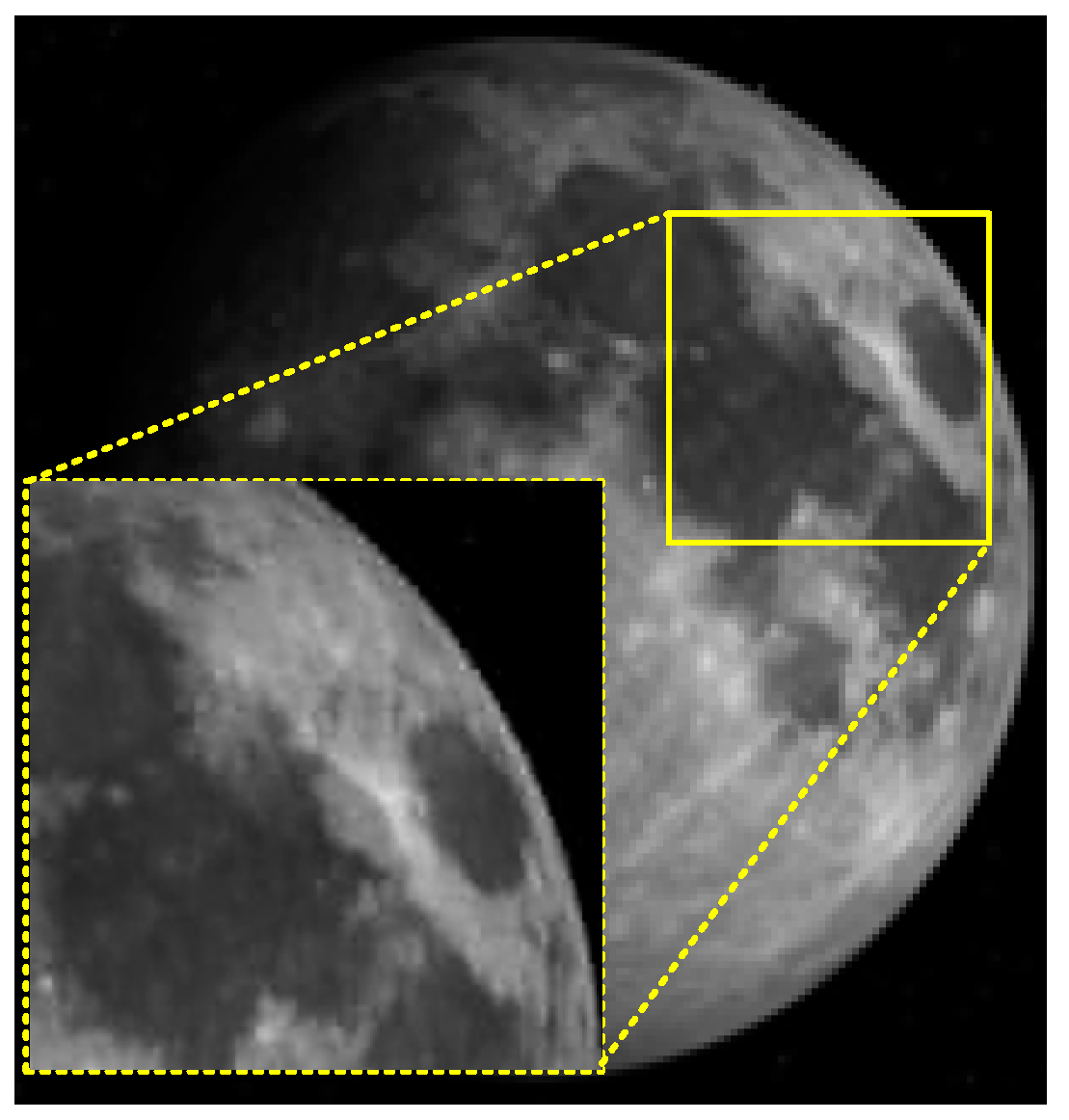
Figure 6.
Part of the reconstructed moon image.
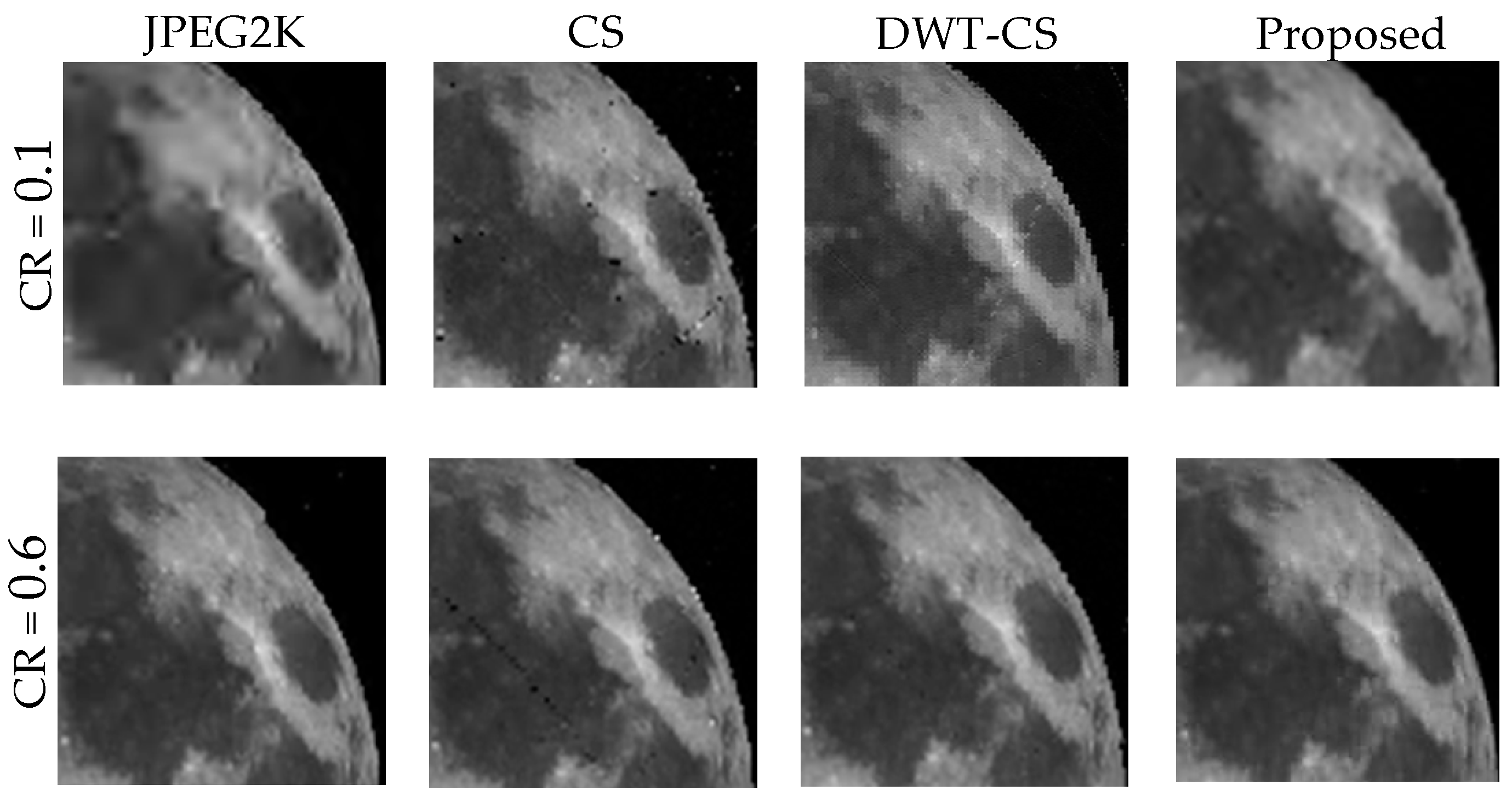
Figure 7.
Planetary images and partial enlargements: (a) Jupiter; (b) Mars; and (c) Mercury.

Figure 8.
PSNR (in dB) comparison of algorithms on planetary images: (a) Jupiter; (b) Mars; and (c) Mercury.
Figure 8.
PSNR (in dB) comparison of algorithms on planetary images: (a) Jupiter; (b) Mars; and (c) Mercury.

Figure 9.
PSNR (in dB) comparison of algorithms on planetary images: (a) Jupiter; (b) Mars; and (c) Mercury.
Figure 9.
PSNR (in dB) comparison of algorithms on planetary images: (a) Jupiter; (b) Mars; and (c) Mercury.


Table 1.
Total number of vectors and their lengths for an image.
| Level | 2 | 3 | 4 | 5 | 6 |
|---|---|---|---|---|---|
| Number of vectors | mn/16 | mn/64 | mn/256 | mn/1024 | mn/4096 |
| Vector lengths | 16 | 64 | 256 | 1024 | 4096 |
Table 2.
PSNR (peak signal to noise ratio) (in dB) comparison based on different algorithms for a range of compression ratio (CR) values applied to a simulation image.
Table 2.
PSNR (peak signal to noise ratio) (in dB) comparison based on different algorithms for a range of compression ratio (CR) values applied to a simulation image.
| CR | ||||||
|---|---|---|---|---|---|---|
| Method | 0.1 | 0.2 | 0.3 | 0.4 | 0.5 | 0.6 |
| JPEG2K | 25.3267 | 27.2289 | 31.5126 | 36.0962 | 43.1136 | 52.8420 |
| Compressed Sensing (CS) | 26.5761 | 28.5148 | 31.0717 | 35.7043 | 42.4761 | 46.2453 |
| DWT-CS | 28.3680 | 30.2784 | 33.9643 | 37.6612 | 44.2360 | 51.5039 |
| Proposed | 30.2346 | 32.1275 | 35.3267 | 41.9209 | 48.0359 | 55.9472 |
Table 3.
SSIM (structural similarity) comparison based on different algorithms for a range of CR values applied to a simulation image.
Table 3.
SSIM (structural similarity) comparison based on different algorithms for a range of CR values applied to a simulation image.
| CR | ||||||
|---|---|---|---|---|---|---|
| Method | 0.1 | 0.2 | 0.3 | 0.4 | 0.5 | 0.6 |
| JPEG2K | 0.7810 | 0.7998 | 0.8355 | 0.8759 | 0.9196 | 0.9810 |
| CS | 0.7902 | 0.8098 | 0.8309 | 0.8646 | 0.9150 | 0.9617 |
| DWT-CS | 0.8004 | 0.8352 | 0.8583 | 0.8802 | 0.9284 | 0.9786 |
| Proposed | 0.8135 | 0.8490 | 0.8618 | 0.9028 | 0.9680 | 0.9987 |
Table 4.
PSNR (in dB) comparison based on different algorithms for a range of CR values applied to moon image.
Table 4.
PSNR (in dB) comparison based on different algorithms for a range of CR values applied to moon image.
| CR | ||||||
|---|---|---|---|---|---|---|
| Method | 0.1 | 0.2 | 0.3 | 0.4 | 0.5 | 0.6 |
| JPEG2K | 21.6909 | 24.4795 | 26.9634 | 29.5922 | 33.6692 | 35.1282 |
| CS | 24.2437 | 26. 2524 | 28.0572 | 30.1587 | 32.9893 | 34.8554 |
| DWT-CS | 25.8281 | 27.8570 | 29.2517 | 32.4487 | 34.3943 | 35.3095 |
| Proposed | 28.9721 | 31.5847 | 33.9489 | 34.7856 | 35.9889 | 37.0392 |
Table 5.
SSIM comparison based on different algorithms for a range of CR values applied to moon image.
Table 5.
SSIM comparison based on different algorithms for a range of CR values applied to moon image.
| CR | ||||||
|---|---|---|---|---|---|---|
| Method | 0.1 | 0.2 | 0.3 | 0.4 | 0.5 | 0.6 |
| JPEG2K | 0.6476 | 0.6994 | 0.7455 | 0.7942 | 0.8698 | 0.8969 |
| CS | 0.6950 | 0.7323 | 0.7657 | 0.8047 | 0.8572 | 0.8918 |
| DWT-CS | 0.7244 | 0.7620 | 0.7879 | 0.8472 | 0.8833 | 0.9002 |
| Proposed | 0.7827 | 0.8312 | 0.8750 | 0.8905 | 0.9128 | 0.9323 |
Table 6.
SSIM comparison based on different algorithms for a range of CR values applied to planet images.
Table 6.
SSIM comparison based on different algorithms for a range of CR values applied to planet images.
| CR | |||||||
|---|---|---|---|---|---|---|---|
| Method | Planet | 0.1 | 0.2 | 0.3 | 0.4 | 0.5 | 0.6 |
| JPEG2K | Jupiter | 0.6648 | 0.7193 | 0.7943 | 0.8641 | 0.8862 | 0.9012 |
| Mars | 0.6935 | 0.7412 | 0.7822 | 0.8438 | 0.8910 | 0.9272 | |
| Mercury | 0.6231 | 0.7081 | 0.7765 | 0.8140 | 0.8742 | 0.9181 | |
| CS | Jupiter | 0.6762 | 0.7457 | 0.8163 | 0.8660 | 0.8900 | 0.9132 |
| Mars | 0.6942 | 0.7553 | 0.8044 | 0.8570 | 0.8783 | 0.9078 | |
| Mercury | 0.6555 | 0.7394 | 0.7841 | 0.8222 | 0.8876 | 0.9307 | |
| DWT-CS | Jupiter | 0.7063 | 0.7911 | 0.8271 | 0.8713 | 0.8955 | 0.9369 |
| Mars | 0.7420 | 0.7891 | 0.8293 | 0.8612 | 0.8852 | 0.9644 | |
| Mercury | 0.6721 | 0.7741 | 0.8316 | 0.8626 | 0.8930 | 0.9497 | |
| Proposed | Jupiter | 0.7884 | 0.8112 | 0.8680 | 0.9019 | 0.9386 | 0.9697 |
| Mars | 0.7700 | 0.8180 | 0.8436 | 0.8845 | 0.9281 | 0.9874 | |
| Mercury | 0.7291 | 0.8050 | 0.8504 | 0.8819 | 0.9218 | 0.9636 | |
Publisher’s Note: MDPI stays neutral with regard to jurisdictional claims in published maps and institutional affiliations. |
© 2021 by the authors. Licensee MDPI, Basel, Switzerland. This article is an open access article distributed under the terms and conditions of the Creative Commons Attribution (CC BY) license (http://creativecommons.org/licenses/by/4.0/).
Share and Cite
MDPI and ACS Style
Zhang, Y.; Jiang, J.; Zhang, G. Compression of Remotely Sensed Astronomical Image Using Wavelet-Based Compressed Sensing in Deep Space Exploration. Remote Sens. 2021, 13, 288. https://0-doi-org.brum.beds.ac.uk/10.3390/rs13020288
AMA Style
Zhang Y, Jiang J, Zhang G. Compression of Remotely Sensed Astronomical Image Using Wavelet-Based Compressed Sensing in Deep Space Exploration. Remote Sensing. 2021; 13(2):288. https://0-doi-org.brum.beds.ac.uk/10.3390/rs13020288
Chicago/Turabian StyleZhang, Yong, Jie Jiang, and Guangjun Zhang. 2021. "Compression of Remotely Sensed Astronomical Image Using Wavelet-Based Compressed Sensing in Deep Space Exploration" Remote Sensing 13, no. 2: 288. https://0-doi-org.brum.beds.ac.uk/10.3390/rs13020288
Note that from the first issue of 2016, this journal uses article numbers instead of page numbers. See further details here.