Research on a mmWave Beam-Prediction Algorithm with Situational Awareness Based on Deep Learning for Intelligent Transportation Systems

Abstract

Simply speaking, automatic driving requires the calculation of a large amount of traffic data and, finally, the obtainment of the optimal driving route and speed. However, the key technical difficulty is the obtainment of data; thus, radar has become an indispensable hardware for automatic driving. Compared to the optical and infrared radar, millimeter-wave radar is not affected by the shape and color of the target, and it is not affected by the atmospheric turbulence, compared to ultrasonic, and so it has a stable detection performance and good environmental adaptability. It is little affected by changes in the weather, and the external environment, rain, snow, dust, and sunshine have no interference in it. The Doppler frequency shift is large, and the accuracy of the relative velocity measurement is improved. However, one challenge for vehicles in fast environments is millimeter-wave-based communication. Because of the short wavelength of the millimeter wave and the high path and penetration losses, the beamforming technology of a large-scale antenna array plays a key role in the construction and maintenance of millimeter-wave communication links. Millimeter waves have wide channel bandwidths, unique channel characteristics, and hardware limitations, and so there are many challenges in the direct use of beamforming technology in millimeter-wave communication. Traditional beam training cannot meet the requirements of low overhead and low delay. This paper, in order to obtain beam information, introduces the context-awareness module to the deep-learning net, which is derived from past observation data. This paper establishes a model that contains the receiver and the surrounding vehicles to perceive the environment. Then, a long short-term memory (LSTM) neural network is used to foresee the acquired power, which is quantized by several beam powers. According to the conclusion, the prediction accuracy is greatly increased, and the model could yield throughput with almost zero overhead and little performance loss.

1. Introduction

One of the most challenging aspects of automotive applications is the configuration of mmWave antenna arrays. Because of its high mobility, the vehicle will be intermittently blocked by other objects during driving, which results in blind spots that are covered by beams. To maintain a high-speed transmission link, the solution is to use frequent beam alignment. Two requirements for the transmission link in in-vehicle applications are low overhead and low latency, and the solutions that are currently employed in IEEE802.11ad are insufficient to meet these requirements [1,2]. However, the only solution that supports massive data sharing is the millimeter wave, and not only that, but the millimeter wave also has a nonnegligible value for 5G in-vehicle cellular communication and infotainment services [3,4]. Therefore, to realize the rapid configuration of mmWave links, it is necessary to design a low-overhead method with high efficiency and high robustness at the same time.

The utilization of out-of-band side information in mmWave vehicular networks is an alternative approach to simplifying beamforming [5]. There are many sensors, such as GPS, visible light radar, lidar, and other sensors around the vehicle, and information is exchanged between various sensors [6] so that the vehicle has the ability of situational awareness. It can be seen from this that side information exists in various parts of the intelligent transportation system.

In [7], the data of sensors and other systems are not only trained by a millimeter-wave beam, but they are also assisted by out-band information. In [8], it was shown that the sub6 GHz band can be used for beam selection and channel estimation because of the channel consistency between the mmWave and sub6 GHz bands. A beam-alignment scheme is proposed, which is achieved by obtaining effective intelligence from radar signals when configuring and designing the vehicle beam.

A method based on inverse fingerprinting is introduced to select the best pair of beams. Just give the location of the receiver, and the beam arrangement for that location is provided by the infrastructure on the basis of the frequency of occurrences in the dataset for that location [8]. The mmWave beam selection with time-dependent vehicle-movement trajectories is addressed by a structure for yielding 5G MIMO datasets of exploding ray tracing, and deep learning is employed for assisted selection.

The millimeter-wave antenna array has high gain and uses more antennas, which leads to high pilot overhead and computational complexity. In order to solve these challenges, scholars propose the use of the method based on deep learning to realize the channel estimation [9,10,11], and deep learning has great potential to reduce overhead [12]. In Ref. [13], the authors propose a novel machine-learning-based method for concurrent transmission in mmWave vehicle-to-vehicle communications. Such an approach can enable effective analog beam selection and the maintenance of low computational complexity. By combining reconfigurable-intelligent-surface (RIS) technology with downlink multiuser communication, the authors of [14] developed a hybrid beamforming scheme to facilitate the sum-rate performance improvement for RIS-based systems. In order to reduce the overhead, the authors of [15] propose a beam-selection scheme that is based on deep learning that randomly selects some beam measurements, and then uses the machine-learning model to estimate the quality of the entire beam. The performance of this method is obviously constrained by the beam search area, and it cannot make full use of the spatial correlation of the beam quality.

In this paper, we propose a novel machine-learning framework that leverages intelligent situational awareness to assist in mmWave beam-power prediction. In a vehicular environment, moving vehicles are the main moving reflectors in cities. Vehicle Intelligent Situational Awareness, as an aid, corresponds to the acquired power of several beams. One way of making the feedback very low or almost zero is to utilize the car’s position as a feature to foresee the acquired power of the different beams. Messages about safety in dedicated short-range communications (DSRC), or the corresponding functions in cellular systems, can provide us with vehicle-location information. First, different regression models are applied to the strongest beam powers. By using different degrees of situational-awareness results to compare to the results that were obtained by regression, the results show that, as the degree of situational awareness deepens, the accuracy of the prediction will also improve, and full situational awareness can obtain the most accurate prediction. With the help of specific datasets, we investigated the influence of the different quantization parameters of the channel-quality index (CQI) on the results. Studies have shown that dataset statistics determine the optimal parameters, and CQI quantization has little effect on the performance under the premise that the resolution can be guaranteed. Finally, the degree to which the power performance of all pairs of beams is affected by multiple regression was also evaluated. The results show that power-prediction-based beam selection can achieve higher throughput than classification-based beam selection.

2. Database Establishment

2.1. Simulation Setup

In this paper, as is shown in Figure 1, a straight street with two lanes located in a modern city is set as our experimental object. The location of the building is calibrated. A road-side unit with a height of 5 m is deployed on the roadside, and only trucks and cars exist in the whole experimental environment. Channel and beam information comes from Romcom’s Wireless Insite software. Since tall trucks are not blocked, we only simulated the passage of low-altitude trucks, and the best pair of beams is invariably line-of-sight (LOS). The receiver in the yellow box is mounted on top of the low-height car, and the green box represents the RSU. Along the road are some fixed buildings. Vehicles are parked randomly in both lanes, the ratio of trucks to cars is constant, and the vehicle density remains basically the same.

The receiver in the yellow box is mounted on top of the low-height car, and the green box represents the RSU. Along the road are some fixed buildings. Vehicles are parked randomly in both lanes, the ratio of trucks to cars is constant, and the vehicle density remains basically the same.

2.2. Channel Model

The mmWave channel is generated by combining the ray-tracing and geometric-channel models [8]. The paths in mmWave-channel modeling are equivalent to the rays in ray tracing. From this, the strongest L-path information can be obtained: $\{{\varphi }_{\ell }^A,{\varphi }_{\ell }^A,{\varphi }_{\ell }^D,{\varphi }_{\ell }^D,{\tau }_{\ell },{\mathit{a}}_{\ell }\},\ell =\{1,2,\cdots ,L\}$, where $({\varphi }_{\ell }^A,{\varphi }_{\ell }^A)$ stands for the azimuth and the elevation of arrival, and $({\varphi }_{\ell }^D,{\varphi }_{\ell }^D)$ stands for the azimuth and the elevation of departure. Moreover, a stands for the path gain for the i-th ray, and τ stands for the time of arrival. Uniform planar arrays (4 × 2) ($N_t=N_r=8$) are deployed at the transmitter and receiver. We approximately named the channel matrix of the geometric channel model as $\mathit{H}\left[n\right],\hspace{0.17em}n=0,1,\cdots L_c-1$.

$$\mathit{H}\left[n\right]=\sqrt{N_t{N}_r}{{\displaystyle \sum }}_{\ell =1}^{L}g\left(nT-{\tau }_{\ell }\right){\mathit{a}}_r\left({\varphi }_{\ell }^A,{\varphi }_{\ell }^A\right){\mathit{a}}_t^{*}\left({\varphi }_{\ell }^D,{\varphi }_{\ell }^D\right){\mathit{a}}_{\ell },$$

(1)

where g (·) is the pulse-shaping filter; ${\mathit{a}}_r({\varphi }_{\ell }^A,{\varphi }_{\ell }^A)$ is the steering vector on the arrival side of the uniform planar array; ${\mathit{a}}_t^{\ast }({\varphi }_{\ell }^D,{\varphi }_{\ell }^D)$ is the steering vector leaving the measurement; and $T$ is the symbol period. The code groups used in the predictive encoder and combiner are DFT codes. The number of pairs of beams in the dataset is $N_B=N_t{N}_r=64$. The encoded information corresponding to the i-th pair of beams is $({\mathit{w}}_i,{\mathit{f}}_i),\hspace{0.17em}i\in \left\{1,2,\cdots N_B\right\}$. The acquired power (y_i) of the corresponding i-th pair of beams is:

$${\mathit{y}}_i={{\displaystyle \sum }}_{n=0}^{L_C-1}{\left|{\mathit{w}}_i^{*}H\left[n\right]{\mathit{f}}_i\right|}^2,$$

(2)

The beam-power regression-training label is $\mathit{y}=[y_1,y_2,\cdots y_{N_B}]$, and the optimal corresponding beam power is $s=\arg {\max }_i\in \{1,\cdots N_B\}{\mathit{y}}_i$.

2.3. Power Quantization

In mmWave systems, the basic structure cannot receive an accurate value of the acquired power through feedback by the channel after beam scanning.

In general, the results obtained by the infrastructure feedback were conducted only by the quantized CQIs and the corresponding pairs-of-beams indices. Therefore, the simulated continuous acquired power obtained from Equation (2) needs to be quantized before proceeding to the next step, which is denoted by i in the first row of

Table 1. Database and postprocessing.

Database	Postprocessing
Original	$\ell =y_1,\cdots ,y_{N_B}$
CQI	${\ell }_C=Q(y_1),\cdots ,Q(y_{N_B})$
Regressor	${\ell }_r=r(Q(y_1)),\cdots ,r(Q(y_{N_B}))$
Ordered beam	${\ell }_m\left(N\right)=r(Q({\overline{y}}_1)),\cdots ,r(Q({\overline{y}}_M))$

. A large number of scholars have studied the mapping scheme from the acquired power to CQI [16,17]. In long-term evolution (LTE), the UE receives the modulation and coding scheme (MCS), and it transmits blocks reliably through the CQI. More specifically, within the bandwidth of the received CSI signal, when the block error rate in the MCS is lower than 10%, the UE can receive the MCS with the highest accuracy rate. The goal of this experiment is different from the above, since, at this point, our main focus is not on the MCS, but on predicting the beam power. After the beam power is obtained, this information will be regressed on the infrastructure. Therefore, in this paper, the main indicator of the reference-signal-acquired power (RSRP) is the CQI. The quantization scheme in this paper as follows: the quantization scheme is uniform, the upper limit of power is $P_u$, and the lower limit is $P_{\ell }$. The acquired power (P) and the CQI can be described by the following formula:

$$Q\left(p\right)=[\min \left\{\max \right\{\frac{p-P_{\ell }}{r_{CQI}},0\},\frac{P_u-P_{\ell }}{r_{CQI}}\}],$$

(3)

where $r_{CQI}$ represents the CQI granularity and defines the ceiling acquired power ($P_u(CQI=Q(P_u))$) and the floor-level acquired power ($P(CQI=0)$). The quantized power is in the interval $\left[P_{\ell },P_u \right]$. Correspondingly, the inverse process of quantization is given by:

$$r\left(q\right)=r_{CQI}q+P_{\ell },$$

(4)

Since quantization reduces the information entropy, it will produce inevitable errors, and especially when the acquired power exceeds our defined interval ($\left[P_{\ell },P_u \right]$). Therefore, in Section 4, we illustrate how the learning accuracy depends on $P_u$, $P_{\ell }$, and the quantization accuracy. Moreover, the results show that the performance will not be significantly reduced because of the reduction in the quantization accuracy.

3. Learning Model

In this section, our main work is to describe how the experimental scene is encoded, and the method that we use to predict the optical power. In our experiments, the power of any beam, including the strongest and weakest beams, was accurately predicted. Not only that, but our method also works when we use pairs-of-beams indexing.

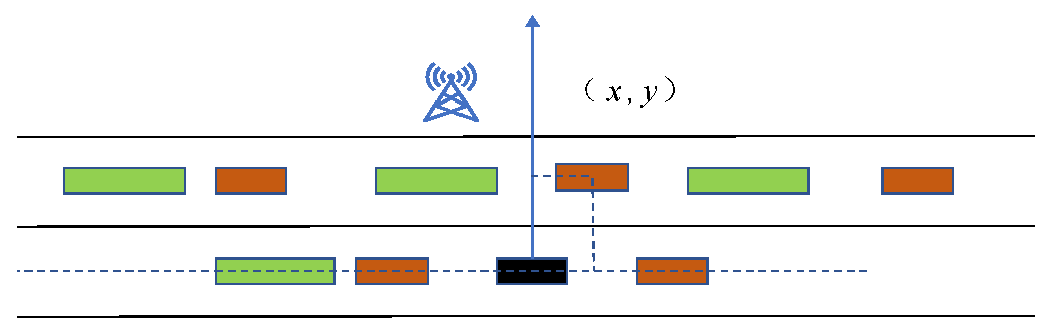
As is shown in Figure 2, the black rectangular box at the origin of the coordinate axis in the figure is the receiver. The longest green rectangle is the aforementioned truck. The remaining brown rectangles are low-height cars.

3.1. Encoding the Geometry

At present, many experts and scholars have conducted a lot of research on vehicle-situational-awareness coding. The environment that was designed for this experiment is two lanes, and there are two types of vehicles. We needed to redesign a vehicle-situational-awareness and coding scheme that is suitable for this experimental environment. First, as shown in Figure 2, we established a Cartesian coordinate system with the receiver’s position as the origin. The unit of the distance is such that all objects can be accurately encoded. For the receiver, the closer a vehicle in the first lane is to the receiver, the more light the vehicle blocks, and the more susceptible is the result. Not only that, although some large trucks are not very close to the receiver, they will also greatly affect the beam of the receiver. Therefore, for the above phenomena, we propose the following encoding and sorting methods to improve the accuracy of the results.

A feature ($v$) of the vehicle can be defined as a vector, which could be described by the following formula:

$$v=\left[\mathit{r},{\mathit{t}}_1,{\mathit{t}}_2,c_1,c_2\right],$$

(5)

where ${\mathit{t}}_1$ and ${\mathit{t}}_2$ represent trucks in the first and second lanes, respectively; $c_1$ and $c_2$ are low-height cars in the first and second lanes, respectively; and $\mathit{r}$ is the vehicle’s position coordinates. The serial number of the car in the first lane is generated in the following way. On the x-axis of the Cartesian coordinate system, the order of trucks along the x-axis is defined as $[x_1,x_2,\cdots x_n]$, and so ${\mathit{t}}_1$ is composed of all the trucks located in the first lane:

$$\begin{array}{c}{\mathit{t}}_1=\left[x_{i_1},y_{i_1},x_{i_2},y_{i_2},\cdots x_{i_N},y_{i_N}\right],\\ \left|x_{i_1}\right|<\left|x_{i_2}\right|<\cdots <\left|x_{i_N}\right|,\end{array}$$

(6)

where N is the maximum value of one type of vehicle in each lane. This maximum value was limited by us in order to keep the dimensionality of the feature unchanged in different scenarios. Provided that the number of trucks in the actual environment is n > N, when encoding, we will remove the redundant trucks with long distances to the feature point. In the same way, if the number of trucks in the actual environment is n < N, we will add some virtual trucks to the spare places. These spare places are generally far from the feature point. In this way, the vehicles in all lanes will be accurately encoded.

3.2. Practical Issues with Feedback

Only a small amount of pairs-of-beams information is transmitted by the feedback link in practice, of which the optimal acquired power of the M beam and the sequence number of it occupy a large part. Because of limited information as to the power of the pairs of beams, we rearranged the order of the pair in descending order (i.e., ${\overline{y}}_1>{\overline{y}}_2>,\cdots ,>{\overline{y}}_M\cdots >{\overline{y}}_{N_B}$). As is seen in Section 4 of Table 1, the regressor is only applied to the acquired power of the first M beam. This model greatly reduces the need for feedback information for all beams, and other methods, such as ordering the beams, can be utilized to achieve lower computational costs. In this article, we only analyze the pairs of beams with the highest power: M = 1.

As is shown in the top row of Table 1, this paper considers the feedback that the infrastructure needs in order to receive the power of the out-of-order beam. It takes a long time to complete the establishment of the database. By building on a comprehensive understanding of the beam power before evaluating the merits of the system, this paper provides a practical method to select the best pairs of beams from an image.

3.3. Main Idea

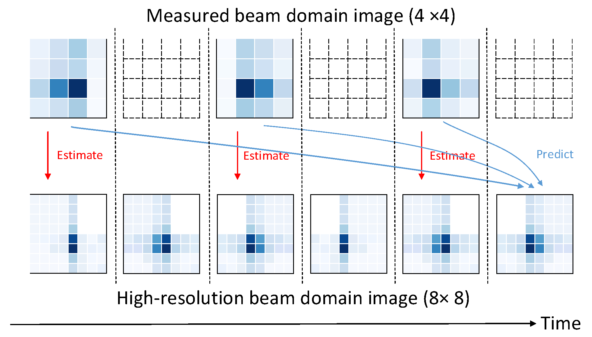
The acquired power that is produced by a uniformly arranged beam can be considered as the image. Through this, low-resolution and high-resolution beam images can be seen as the gain powers of wide and narrow beams, respectively. The use of wide beam measurements to measure the beam quality of narrow beams is the main idea of the model. Thus, the goal that we aim for is to apply the super-resolution onto the beam-domain images. By combining the two models, the proposed beam-selection method is constructed. One is a model that estimates the quality of the beam, and the second is an estimation model that is based on predictions. The study of the first model is on the difference between low-resolution and high-resolution beams in the beam domain, and the output of the second model is the current high-resolution image of the laser in the beam domain, which requires some empirical values. At regular intervals, the receiver receives an uplink pilot signal.

According to the uploaded signal, the BS can estimate the quality of the current beam, and it can also predict the beam quality within the coherence time of the next channel. Figure 3 shows the envisioned scheme framework for beam selection for high-resolution beamfield images and low-resolution images, in turn, and the unroll predictions from multiple low-resolution images, since the predicted result reduces the number of measurements per unit time, which means a reduction in the overhead, in turn. The goal is to acquire correlations in the spatial domain in images, and both models employ CNN techniques to achieve super-resolution. In addition, the prediction model in this paper adopts the deep-learning algorithm that is borrowed from the LSTM network, and by considering the time relationship of the beam quality, the computational cost is further optimized. In order to preserve useful information, the LSTM extracts the variation in the beam in the time domain, which can foresee the current quality value of the beam from the previous beam-measurement values. The rest of this section will cover the estimation and the prediction of the beam quality in detail.

3.4. Model to Estimate the Beam Quality by Deep Learning

The proposed system not only measures the received up-pass frequency signal of each broad beam, but it also builds a beam-domain image without high resolution. The inputs to the machine-learning-based model are images that present the acquisition power and the wide beam. The learning framework that is envisaged in this paper outputs input data with high resolution onto the beamfield image that represents the acquired power, as well as the narrow beam.

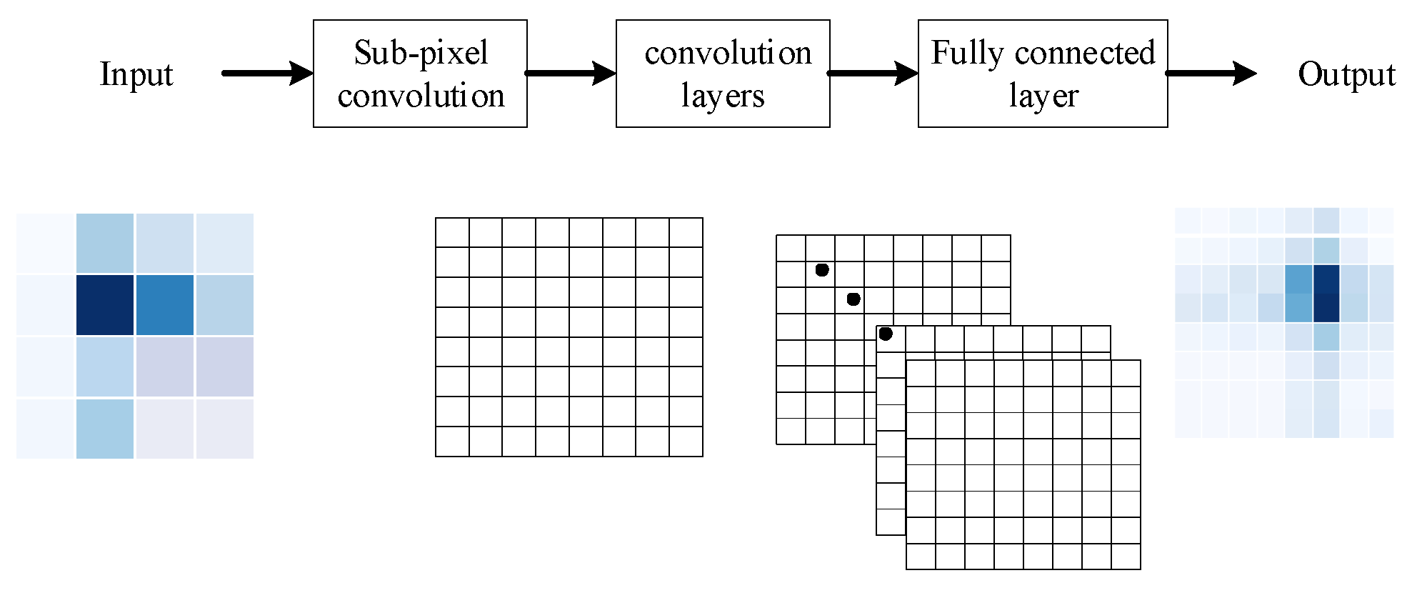
A model is used to estimate the power of the received narrow beam whenever an upstream frequency signal is received. The construction of the model that is referred to is shown in Figure 4. As is shown in Figure 4, a 2D convolutional layer and a convolutional layer with subpixel upsampling are used, before the input to a normal convolutional layer. A powerful super-resolution technique is used in these two layers, which can learn to improve the fractional variability in the picture. Subpixel convolution can reduce the computational complexity and can upgrade maps by using complex filters that are trained with special inputs. This information can be used to increase the resolution of the image through the upsampling layers. As described above, two 2D convolutional layers make up the subnetworks below. Spatial correlations in images can be used by these layers. Thanks to the specific input type that was designed, the acquired power of the wide beam depends on the beam direction. The fully connected (FC) layer is the last layer of the neural network. As you can see,

Table 2. Architecture of the estimation model.

Layer Type	Filters	Filter Size	FC Neurons
Conv 2D	4	(3,3)	-
Sub-pixel Conv 2D [18]	-	-	-
Upsampling 2D [19]	-	(2,2)	-
Conv 2D	40	(3,3)	-
	40	(3,3)	-
Flatten	-	-	-
Dense	-	-	128
			64

shows the number of neurons in the fully connected layer, each layer of the neural network, and the size of the filter. Our proposed scheme uses a trained model to estimate high-resolution beamfield images, and it chooses the narrow beam that obtains the highest energy.

3.5. Model to Predict the Beam Quality by Deep Learning

In this paper, in order to reduce the training cost, the pilot signal is propagated only once in the coherence time of one channel. By contrast, past pilot signals predict the acquired power of the current narrow beam. With this, the training time will be halved. The architecture of the model that was used for prediction is shown in Figure 4. It can be seen that the basic architecture of this model inheritance comes from the estimation model, which means that the convolutional layers of this, as represented in Table 1, have exactly the same parameters and construction. The most fundamental difference between the estimation and the forecasting of models is the tracking of the differences in the time domain by using LSTMs for forecasting models, as Figure 5 shows. The convolution-based LSTM network was used in the prediction model. Both the spatial features that are extracted by the convolution, and the temporal features that are extracted by the LSTM, can be captured at the same time by the convolutional LSTM. A list of pixels is the input to the convolutional LSTM. In this method, in order to capture the variation in the beam quality in the time domain, the L-shaped low-resolution image is input into the prediction model.

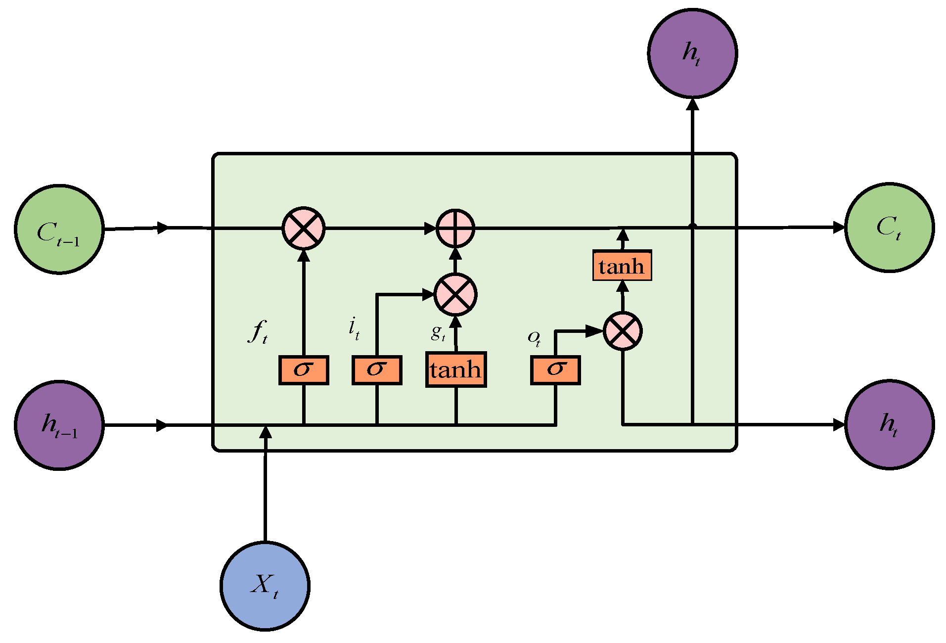
LSTM is a kind of dynamic neural network that solves the problem that the traditional neural network cannot, which is to adaptively use the past data. LSTM is a special RNN with the ability to learn long-term dependency, and its structure is shown in Figure 6.

The repeating module in an LSTM cell contains four interacting layers: a forgetting gate layer ($f_t$), an input gate layer ($i_t$), an output gate layer ($o_t$), and a new candidate layer ($C_t$). In the LSTM net structure, the gate is realized by a sigmoid function, and the forward propagation mathematical model of the LSTM neural network is as follows:

$$\begin{array}{c}{f}_t=\sigma \left(W_f·\left[h_{t-1},x_t\right]+b_f\right),\\ i_t=\sigma \left(W_i·\left[h_{t-1},x_t\right]+b_i\right),\\ {\tilde{C}}_t=tanh\left(W_c·\left[h_{t-1},x_t\right]+b_c\right),\\ C_t=f_t\ast C_{t-1}+i_t\ast {\tilde{C}}_t,\\ o_t=\sigma \left(W_o·\left[h_{t-1},x_t\right]+b_o\right),\\ h_t=o_t\ast tanh\left(C_t\right)\end{array}$$

(7)

where $\sigma$ represents the sigmoid function:

$$\sigma \left(x\right)=1/\left(1+e^{-x}\right)$$

(8)

In the LSTM estimation model, the LSTM layer contains 256 neurons. To enrich this article, the deconvolution layer is used instead of the FC layer in the last part of the network. It is worth noting that the performance of the deconvolution super-resolution architecture is almost the same as that of the FC-layer super-resolution architecture in the case of input of different amounts of training data (namely, pixel sequences). However, in the case of deconvolution, the time cost of the training parameters is expensive, and so the training speed of each epoch element is slightly slower.

4. Performance Evaluation

In this section, in order to achieve better prediction results, we use many kinds of learning models and datasets for the regression training in order to find the best results. The relevant metrics are defined by us, and, in order to evaluate the system performance, we use different quantization parameters. Finally, we test the property of the predicted power for each pair of beams.

4.1. Performance Metric Definition

The actual beam power can be expressed as $Y=\{{\mathit{y}}_1,{\mathit{y}}_2,\cdots {\mathit{y}}_m\}$, and the predicted value as $\widehat{\mathbf{Y}}=\left\{{\widehat{\mathit{y}}}_1, \dots {\widehat{\mathit{y}}}_m\right\}$. Then, the alignment-probability expression can be obtained as $P_A=\frac{1}{m}{\displaystyle {\sum }_{i=1}^m(\arg \max ({\mathit{y}}_i)=\arg \max ({\widehat{\mathit{y}}}_i))}$, where max{·} represents the largest element in the vector vector(·); argmax{·} represents the index of max{·}; and (·) is the indicator function. Thus, the throughput rate can be expressed as R_T as:

$$R_T=\frac{{{\displaystyle \sum }}_{i=1}^m{\log }_2(1+{\mathit{y}}_i[\mathrm{argmax}\left\{{\widehat{\mathit{y}}}_i\right\}])}{{{\displaystyle \sum }}_{i=1}^m{\log }_2(1+\max \{{\widehat{\mathit{y}}}_i\})},$$

(9)

The actual throughput RT is only related to the learned model, and not to the beam training.

4.2. Regression Models

The configuration environment is presented in Section 3.1. In this section, we will analyze the different regression models and compare them to the actual results. When quantifying the strongest beam power, we use the root mean square error (RMSE) to determine the quantization regression accuracy, and so the unit is dB. The RMSE can be described by the following formula:

$$\mathrm{RMSE}=\sqrt{\frac{1}{m}{{\displaystyle \sum }}_{i=1}^m{\left({\widehat{\mathit{y}}}_i-{\mathit{y}}_i\right)}^2},$$

(10)

where ${\widehat{\mathit{y}}}_i$ is the predicted beam power; ${\mathit{y}}_i$ is the predicted value; and m is the number of beams.

Table 3. RMSEs of four regression algorithms.

Algorithm	RMSE (dBm)
Random Forest	1.726
Linear Regression	6.199
Gradient Boosting	2.814
SVR	3.645

presents the prediction results of random forest regression, linear regression, gradient boosting regression, and support vector regression. The results show that random forest regression has the best results because it can handle very high-dimensional data without feature selection and, at the same time, the model has a strong generalization ability [20]. Random forest regression also has a fast training speed, and so this method can be widely used in industrial production.

4.3. Different Levels of Situational Awareness

In this section, we discuss the role and the advantages of situational awareness in predicting beam power. The current loss models are only concerned with the relative distance [4], or with the absolute position between the receiver and the transmitter [21]. The authors of [8] also show that there is only one way for the location of the receiver to provide useful information about the beam, and that is through previously transmitted datasets. The experiments in this paper show that, in an urban environment, not only can the dataset provide location information, but there is also a more accurate way to predict the beam power, which is to use the environmental information around the vehicle location for the prediction.

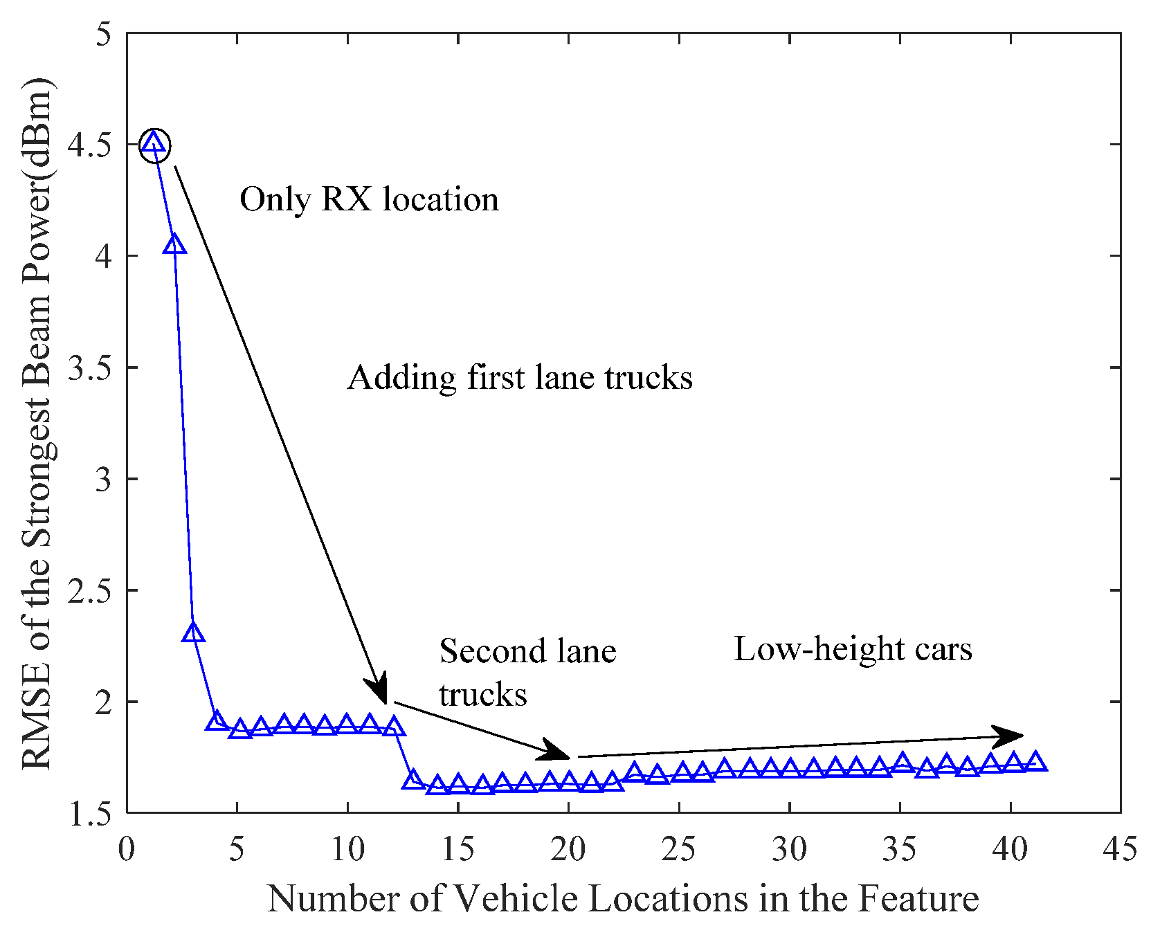
The position information of the vehicle is provided in Section 3.1. Figure 7 shows the RMSEs of the strongest pairs of beams. The prediction method that was used is random forest regression. The dots in the figure represent the positions of the i-th vehicle, as described in Section 3.1. The results show that most of the information on the beam power is provided by the trucks in the first lane. The RMSE is now around 1.7, which is down from 4.5 for the previously described case that used only the receiver as a feature. Meanwhile, the truck position in the second lane lowered the RMSE to 1.6. However, low-altitude cars have little effect on beam-power predictions. Not only that, but when we add other types of vehicles, the RMSE drops slightly, but not to a significant degree. From this it is concluded that the position of the tall truck in the first lane has a very strong correlation to the beam-power prediction. Furthermore, when the lane-location features are not complex, the predicted results will be more accurate.

4.4. CQI Quantization

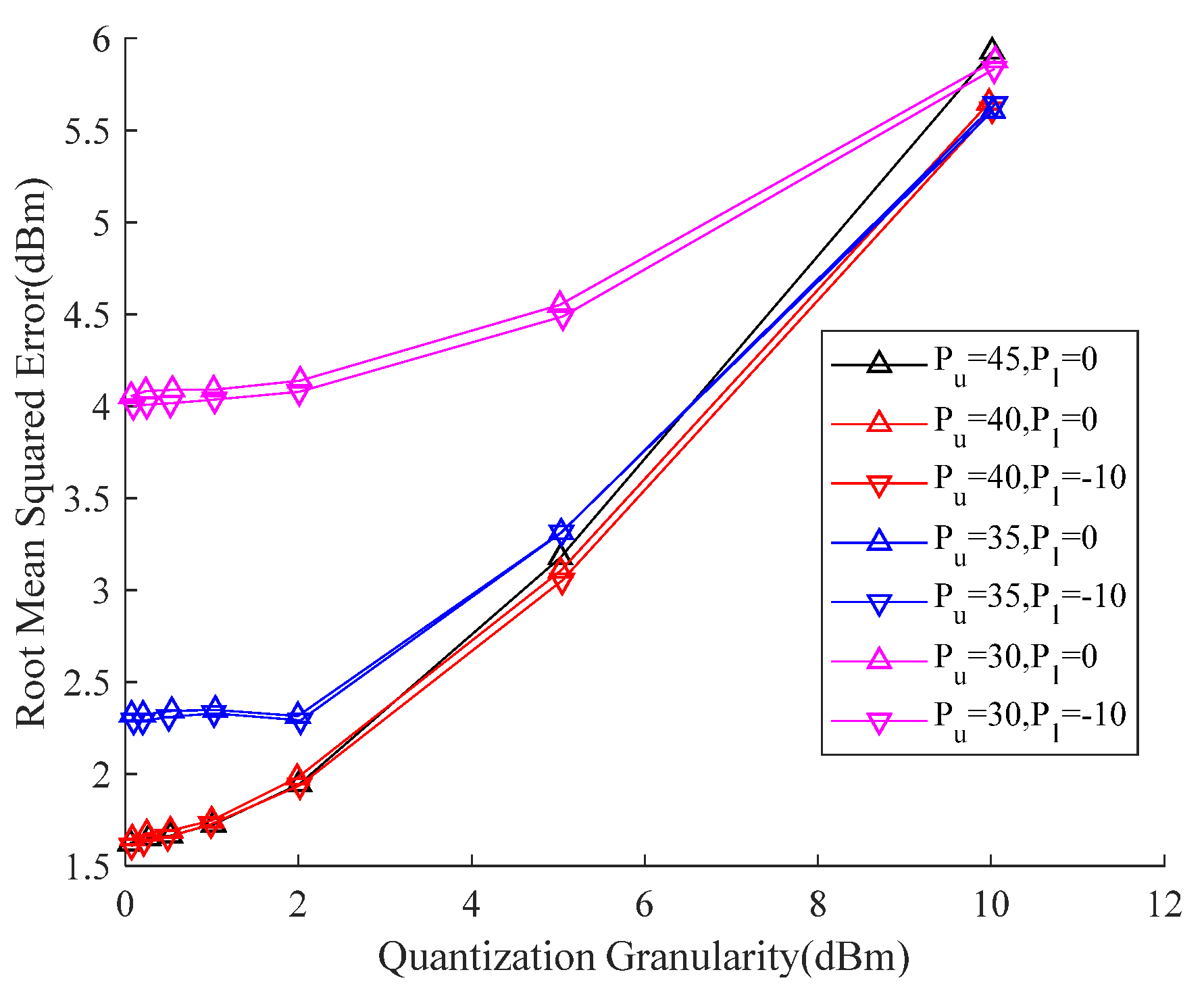
This section discusses the relationship between the CQI-quantization performance and the prediction power of the strongest beam. First, as described in Section 2.3, we quantize the continuous power and restore the quantized power to continuous power. The parameters $r_{CQI}$, $P_u$, and $P$ are used by us in different combinations to evaluate the predicted RMSE. It can be seen from the observation results of the dataset that, among all pairs of beams, the maximum beam power is $P_{\max }=44.23$ dBm, and the minimum beam power is $P_{\min }=-15.15$ dBm. After multiple experimental validations, we chose to use a combination of $P_u$ and $P_{\ell }$ to evaluate the RMSE, as is shown in Figure 8.

The experimental results show that the change in the RMSE is usually accompanied by a large change, and, within a small range of change, the RMSE is basically unchanged, which indicates that the RMSE presents a certain step shape in the change granularity of this experiment. In addition, when the value of $P_u$ is larger, the predicted result is more accurate, but the change in the value of $P_{\ell }$ has little effect on the predicted result. The reason for this phenomenon is that we predict the value of pairs of beams with the strongest power. When the value of the upper bound ($P_u$) is not large enough, it is easy to cause the beam power to be outside the interval ($\left[P_{\ell },P_u \right]$), which thereby causes a large quantization error. Although the lower bound has little effect on the prediction results, we should also carefully design the upper and lower bounds. Only in this way can all the data in the dataset be distributed in the interval ($\left[P_{\ell },P_u \right]$) as much as possible, which thereby minimizes the quantization error.

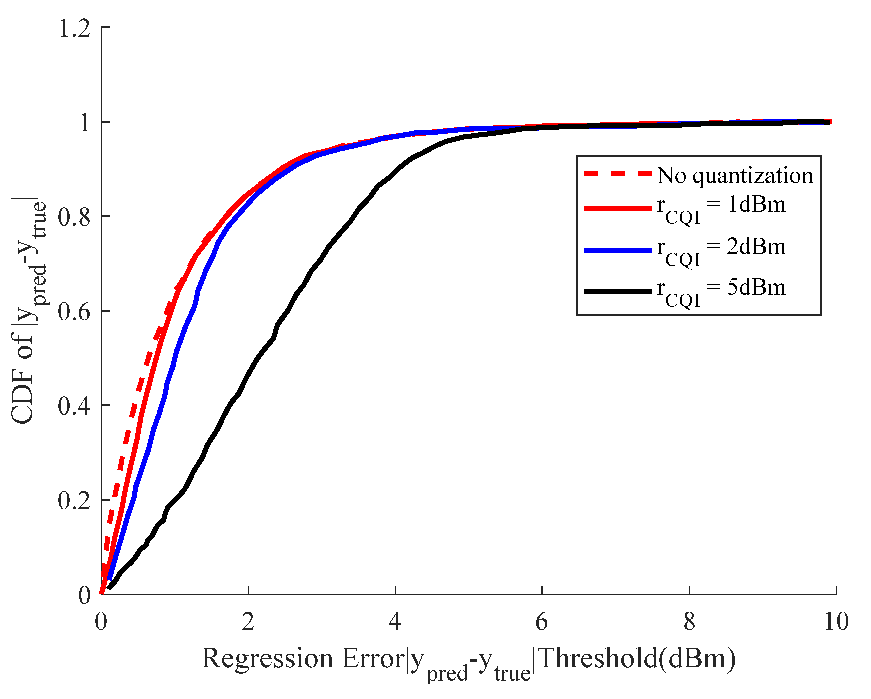
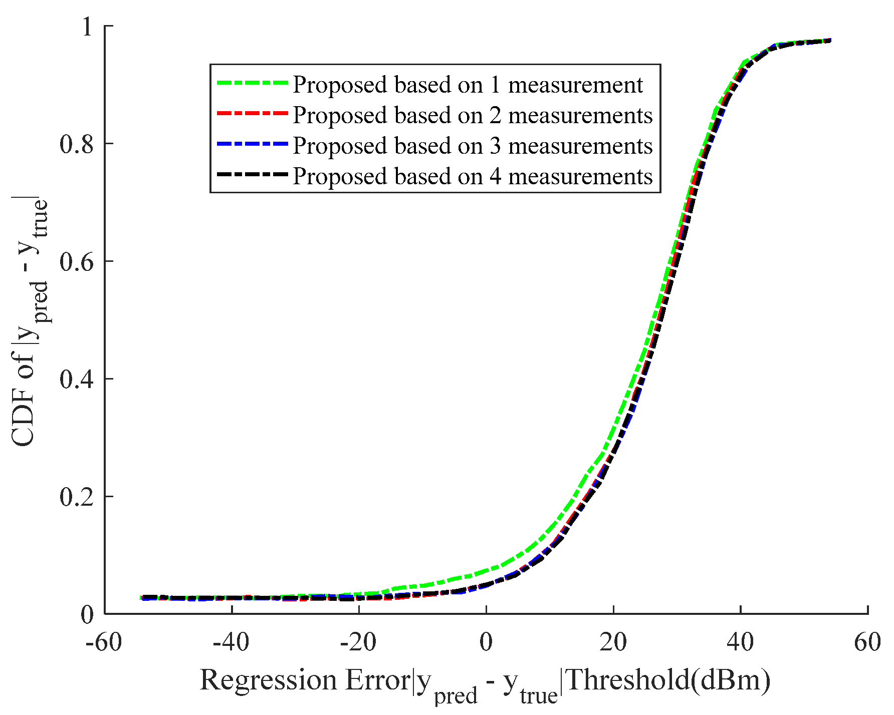
Figure 9 further discusses the cumulative density function (CDF) between the different quantization granularities and the regression errors. The three points on the blue, black, and red lines stand for the probabilities of regression error under 1 dBm for the three $r_{CQI}$ conditions. The experimental results show that when $r_{CQI}$ is 1 or 2 dBm, the predicted error less than 1 dBm can exceed 50%. Moreover, when we use 1 dBm as the quantization precision, the prediction result is not much different from the prediction result without quantization. The reason for this phenomenon may be due to quantization error. When we use actual data, there is no quantization error. In addition, when we use CQI = 1 dbm and 2 dbm, the quantization error is so small that it has little effect on the result.

4.5. Evaluation of Beam-Quality-Prediction Models

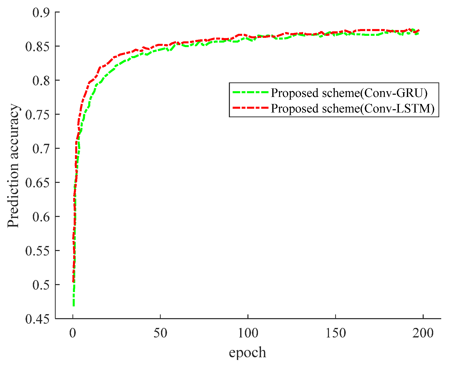
In this section, we evaluate the property of beam selection in consistent time for all of the above schemes, without transmitting the pilot signals. The input to the prediction model is the low-resolution image of the last three pilot signals. Figure 10 shows the CDF of the SNR. As is shown in Figure 10, when using convolutional LSTM (Conv-LSTM) and the convolutional gating unit (Conv-GRU) with our proposed scheme, our SNR is better than that of the no-prediction exhaustive-only approach. The reason is that our scheme has the advantage of capturing the motion state of the UE, so as to predict the acquired power more accurately. Furthermore, our scheme results in little difference in the CDF performance, regardless of whether Conv-GRU or Conv-LSTM is used. The reason for this phenomenon is that both the Conv-RELU and Conv-LSTM neural networks have the function of predicting the current beam measurement from the past beam measurement. Not only that, the SNR of our prediction model is almost identical to that of optimal beam selection; however, our scheme is trained less often, in less time, and with less overhead. Since the other SNRs are almost identical, our scheme can be obtained with high accuracy and reliability. For our proposed scheme, too many or too few input images will affect the prediction performance. Figure 10 shows how the MSE varies with the number of input images. Figure 11 shows the variation in the CDF of the SNR between the two powers. In Figure 10, when the number of input images is more than one, the final SNR is almost unchanged. The reason is that we cannot obtain the velocity information of the object through only one sample. 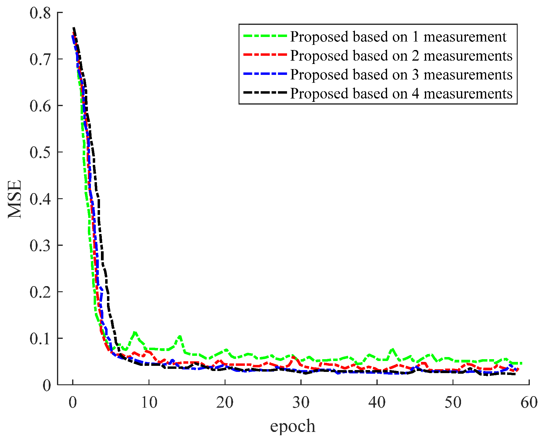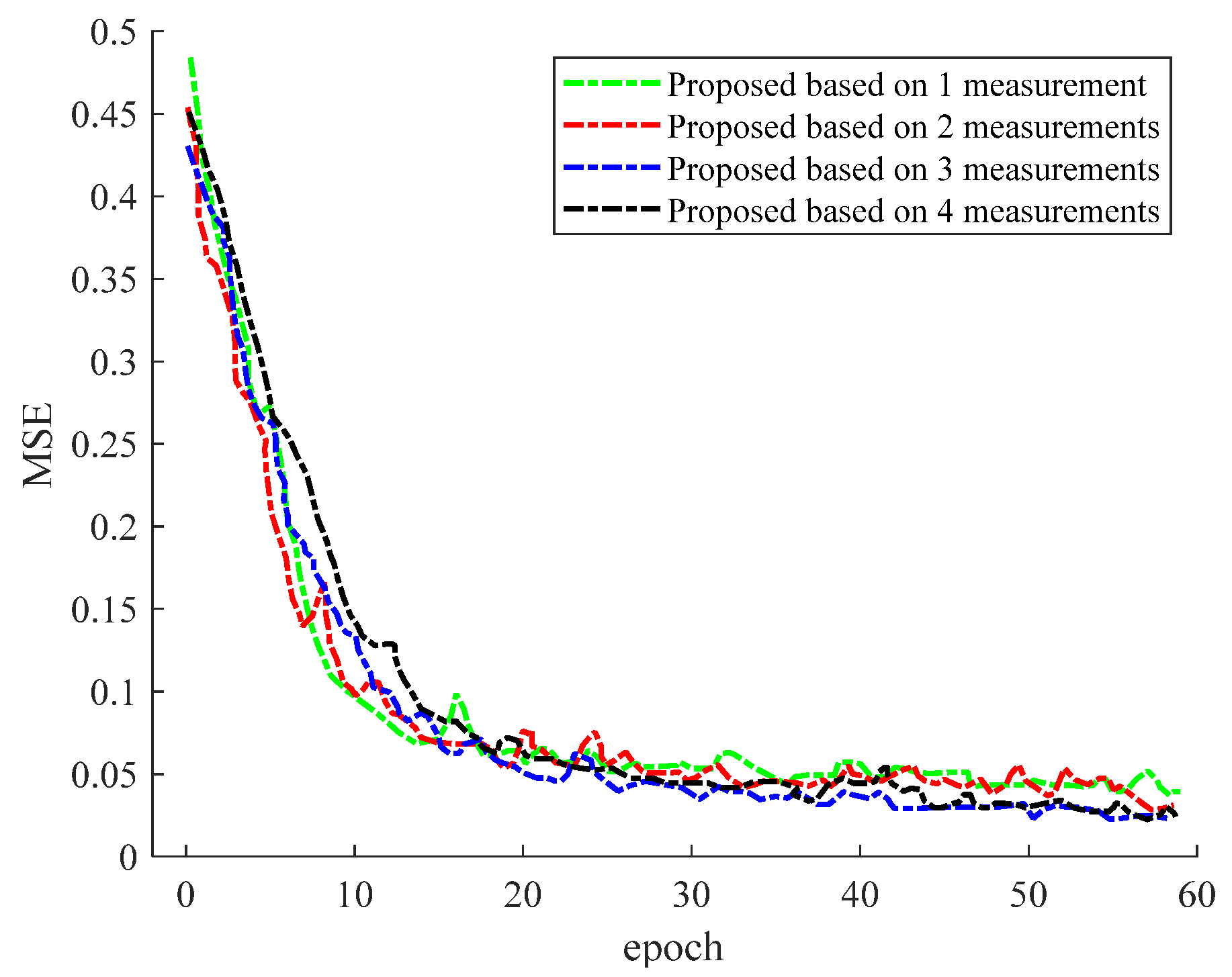As is shown in Figure 11, when we input more image data, the performance of the model after convergence is better. However, it should be noted that, as the input image data increases, the speed of the model convergence becomes slower. This is because, as the input image increases, the corresponding image feature dimension also increases. 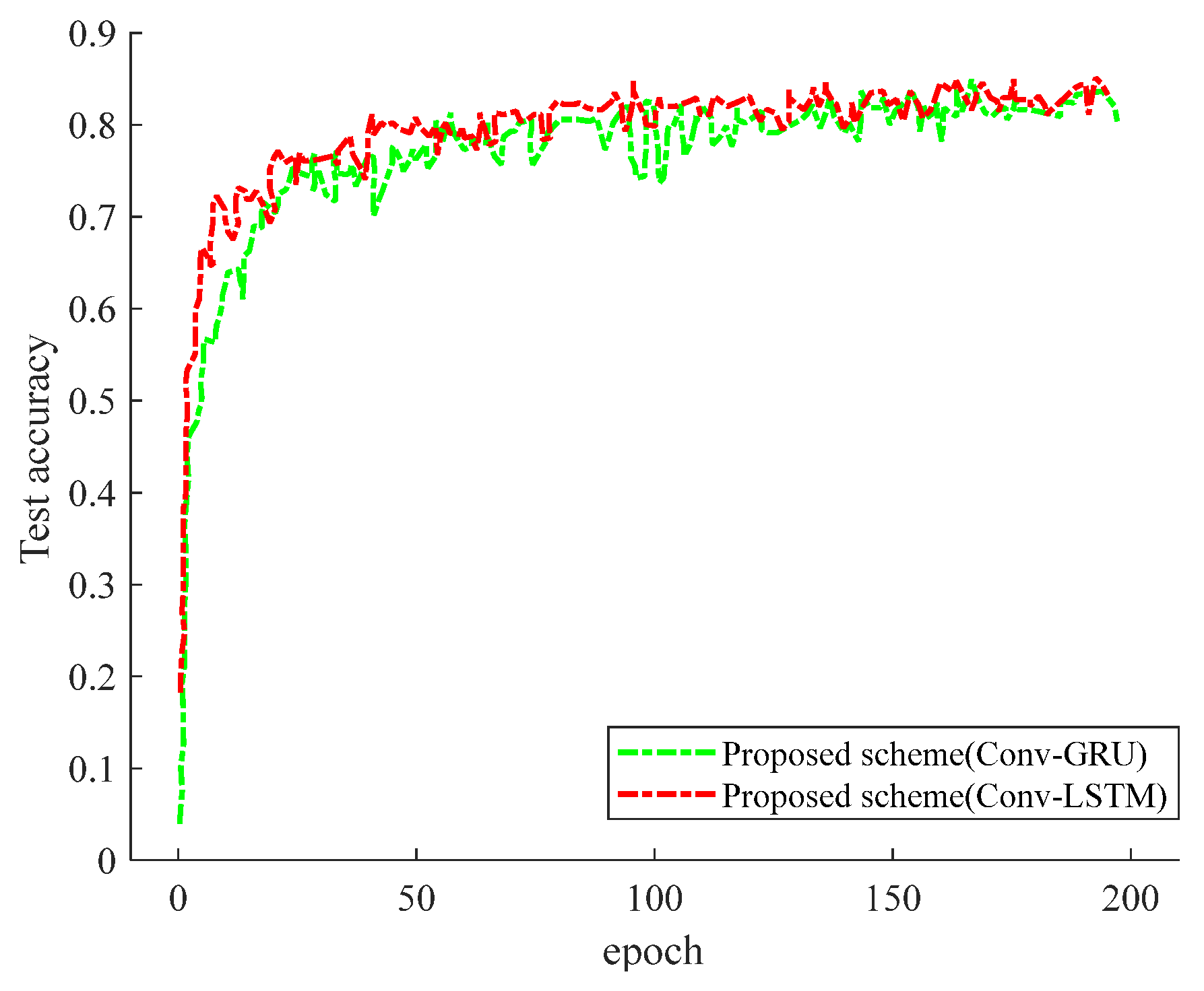Figure 12 shows the MSE performance of our proposed scheme. The scheme uses Conv-GRU, where the different-colored line segments represent different numbers of inputs. The results in Figure 13 and Figure 14 show that, when we adopt Conv-GRU, the prediction performance of the model is better with more input-image data.

5. Conclusions

This paper combines situational-awareness technology and an LSTM neural network to predict beam power to improve the accuracy of the prediction. The results show that the part of our prediction error less than 1 dBm can exceed 50% when the complexity of the road situation is not high. We reduce the number of training times, shorten the processing time, and reduce the overhead, while ensuring a high SNR. Not only that, but our model is also highly robust, and it can handle highly concurrent data well. When the road situation becomes complex, the input data increases accordingly, and the noise interference also increases rapidly. Our model can ensure a higher accuracy rate with a small decrease in the convergence speed. However, when the road conditions are complicated enough, our model may not work. Our method has the characteristics of high efficiency, high robustness, and low overhead, which can meet the fast configuration requirements of mmWave links in autonomous driving, and it has great industrial value.