Non-Intrusive Monitoring Algorithm for Resident Loads with Similar Electrical Characteristic

1
Department of Engineering, Electric and Electronical Engineering, University of Strathclyde, Glasgow G1 1XW, UK
2
Department of Engineering, Electric and Electronical Engineering, University of Strathclyde, Glasgow G1 1RX, UK
*
Author to whom correspondence should be addressed.
Processes 2020, 8(11), 1385; https://0-doi-org.brum.beds.ac.uk/10.3390/pr8111385
Submission received: 7 September 2020
/
Revised: 11 October 2020
/
Accepted: 19 October 2020
/
Published: 30 October 2020
(This article belongs to the Special Issue Power System Expansion Planning)
Abstract
:Non-intrusive load monitoring is a vital part of an overall load management scheme. One major disadvantage of existing non-intrusive load monitoring methods is the difficulty to accurately identify loads with similar electrical characteristics. To overcome the various switching probability of loads with similar characteristics in a specific time period, a new non-intrusive load monitoring method is proposed in this paper which will modify monitoring results based on load switching probability distribution curve. Firstly, according to the addition theorem of load working currents, the complex current is decomposed into the independently working current of each load. Secondly, based on the load working current, the initial identification of load is achieved with current frequency domain components, and then the load switching times in each hour is counted due to the initial identified results. Thirdly, a back propagation (BP) neural network is trained by the counted results, the switching probability distribution curve of an identified load is fitted with the BP neural network. Finally, the load operation pattern is profiled according to the switching probability distribution curve, the load operation pattern is used to modify identification result. The effectiveness of the method is verified by the measured data. This approach combines the operation pattern of load to modify the identification results, which improves the ability to identify loads with similar electrical characteristics.
1. Introduction
With the continuous improvement of living standards across the world, residential power consumption has rapidly increased [1]. More and more transmission and distribution equipment overload operation, which shortens equipment’s service life [2]. Effective residential load management can relieve overloading of the power equipment, but it can also enhance the operation efficiency and stability of the power grid and improve energy utilization. Load monitoring technology is core to load management schemes; it can obtain the power consumption information of each load, provide feedback power data to grid managers, and help residents improve their own electricity consumption patterns, reducing their electricity bills. Load monitoring technology can obtain the operation status and power consumption details of each load. The obtained power consumption information can be used in various areas: firstly, the grid managers can provide residents with clear and transparent load power consumption list, which is effective for residents to reasonably arrange the load using time. Secondly, residents can adjust and optimize their power consumption pattern according to the power consumption list and energy saving suggestions provided by the grid manager, so as to achieve the purpose of saving energy and electricity charges. In addition, the detailed power information includes each load energy efficiency, it can promote the research and development process of low energy consumption equipment by the electrical appliance manufacturer.
The traditional approach of load monitoring is intrusive in terms of style, in that it installs a sensor with each load to record energy consumption information and power data. Traditional methods can maintain high monitoring accuracy and reliability, but they are impractical as the implementation cost is high and it is significantly inconvenient for residents. To overcome the mentioned problem, non-intrusive load monitoring (NILM) technology was proposed in the early 1980s [3]. NILM technology involves the installation of data-acquisition devices at the electrical supply entry points among residents to obtain the total electrical current (signal). The signal is processed by signal processing techniques to analyze changes in the current going into a residence and deduce what appliances have been switched on/off. NILM technology only uses one data-acquisition device, which makes signal acquisition fast, though monitoring accuracy is decreased when data-acquisition devices are used less. The main research direction here is how to maintain high monitoring accuracy with a non-intrusive style.
More recently, the research direction of NILM focuses on load identification and decomposition algorithms. In reference [4], seven kinds of steady-state load characteristics are selected to train a feature mapping neural network so that load identification can be realized based on the trained neural network. In reference [5], active power, reactive power and power factor are combined to form a load feature group, and the k-nearest neighbor (KNN) algorithm is used for load identification. Reference [6] combines steady-state characteristics with transient waveforms to decompose and identify load types. In reference [7], researchers train a neural network using the harmonic wave from the first to the eighth order, which is then used to identify the load. In reference [8,9,10], wavelet coefficients are used to represent load characteristics to train a neural network, improving the accuracy of load identification. Reference [11] treats the current harmonic as the training feature and trains the weights of the neural network by means of a particle swarm optimization method to improve the recognition accuracy. Reference [12] analyzes the structure of electrical equipment and establishes a special feature library for each piece of electrical equipment, thereby training the neural network for load identification. In reference [13], the frequency characteristics of the load is analyzed by Hilbert transform to realize load identification. Reference [14] and reference [15] take the characteristics of load trajectory and front-end circuit topology, respectively, as auxiliary features for load identification.
According to the survey in the current paper, the published load identification methods are based mainly on load electrical characteristics, but if the electrical characteristics of the loads were remarkably similar, these published load identification algorithms would be difficult to maintain with a high identification accuracy [16]. In terms of detecting discrepancies between electrical characteristics between loads, the identification process is better, and one such distinctive discrepancy is the pattern of the load operation. This is because the switching probability varies between different loads. This paper proposes a method to improve the identification results based on load operation patterns. Firstly, the load decomposing algorithm is used to obtain the working current signal of a load. Secondly, the working current signal of the load is processed based on the KNN algorithm, and load type and running period are identified. Thirdly, based on the identification results, load switching times in each period are counted. A back propagation (BP) network is trained with the counted results, and following that, the BP network is used to fit the operation pattern curve of the identified load. Finally, the operation pattern curve is analyzed to improve results.
The current paper used test data recorded from one house. The recorded data include two parts, one is sampled from the whole-house voltage and current at 16 kHz, having calculated the active power, apparent power and RMS (Root Mean Square) voltage. The data is also sampled at the single home appliance side, voltage and current are sampled at 10 kHz, obtaining the switching event node of the home appliance and providing reference for the experiment results. In this way, the study recorded the active power drawn by individual appliances and the whole-house apparent power demand. Furthermore, the study recorded power data of every single appliance in the house individually. The test results show that the proposed method can effectively improve the identification accuracy of loads with similar electrical characteristics.
2. Fundamental of NILM
NILM treats the voltage and/or current signal at the home’s electrical supply entry point as the monitoring target. By analyzing the monitored mixed signals, NILM can achieve monitoring of various load states independently, as well acquiring each load power consumption information. Through the acquisition of detailed operation information data of each load within the user, it can provide more accurate data for the power grid to achieve load forecasting, improve the accuracy of power load forecasting, and provide more accurate data for power system simulation analysis, system planning and security and stability guarantee of power grid lines.
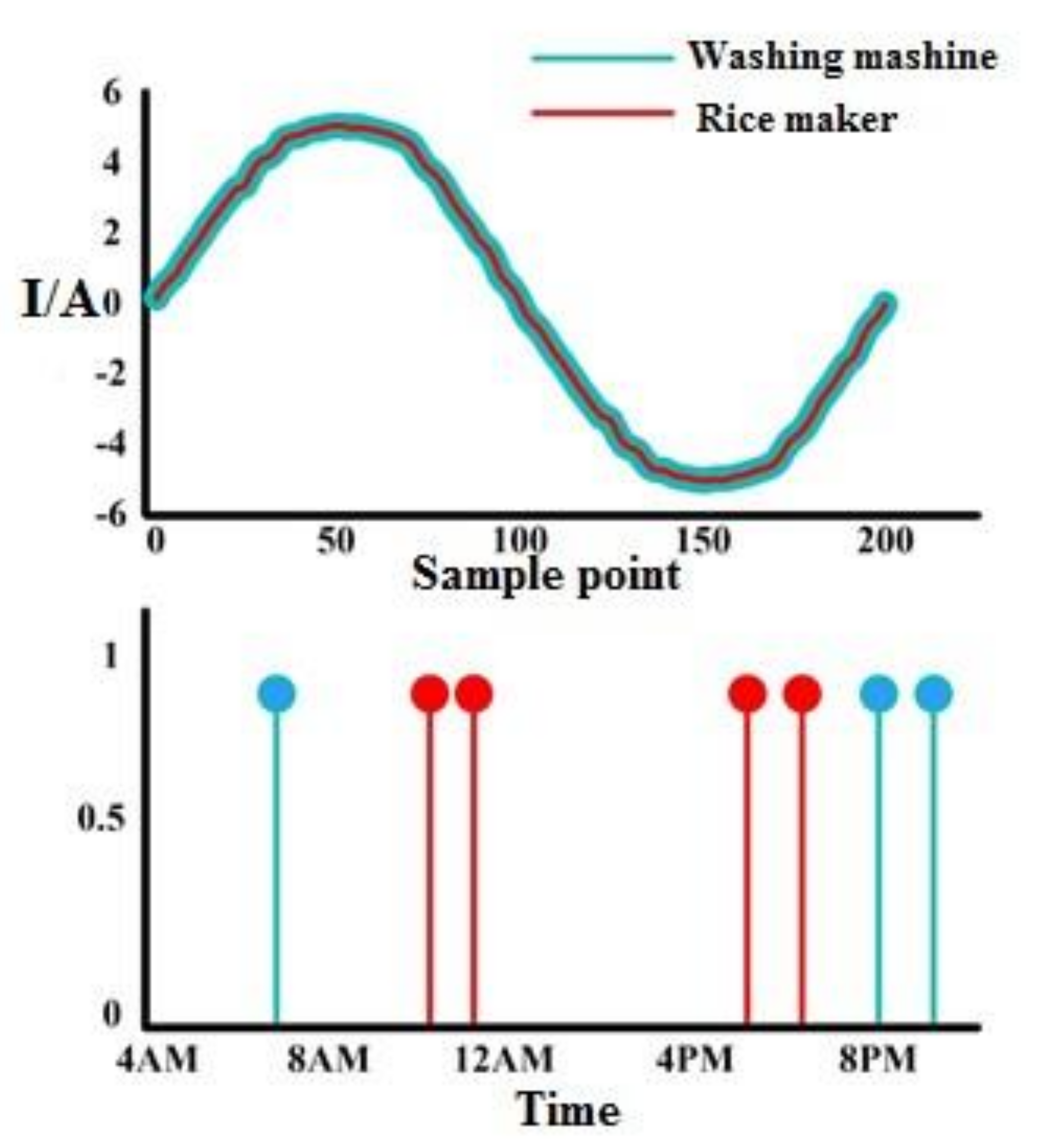
In the process of power consumption information extracting and load state monitoring, selection of load electrical characteristic is vital in this process, which deeply affects the accuracy of NILM. However, no matter how one selects the electrical characteristic, the overlapping of characteristics between the loads is unavoidable, and as an example, the working currents (signals) of the rice cooker and the washing machine shown in Figure 1 are almost the same. As such, the electrical characteristics of the two loads are similar, so the accuracy of the results from the load identification algorithm are likely to be affected. On the other hand, two appliances have different operational regularities, and the rice cooker is most likely to be used around 12:00 p.m. and/or 6:00 p.m., while the washing machine is likely to be used around 7 a.m. and/or 8 p.m. Therefore, switching probability distribution curves for the rice cooker and the washing machine are rather different. If the rice cooker and washing machine were to be identified based on their electrical characteristics, incorrect identification would occur, but analyzing the operation regularity of the two loads can improve the identification results.
In the above mentioned example, a new method of NILM is proposed to improve the identification accuracy of loads with similar electrical characteristics.
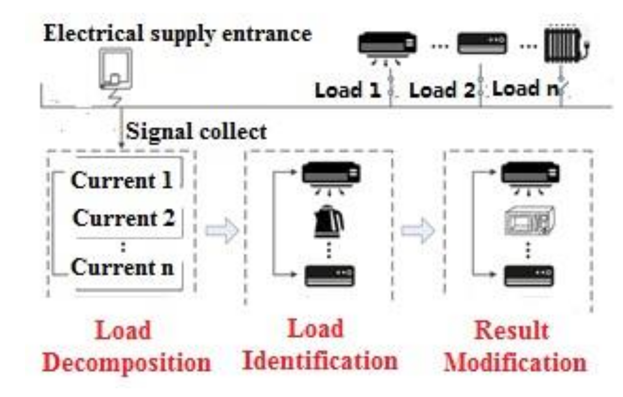
The overall implementation structure of this method is shown in Figure 2. The method is divided into three parts: load decomposition, initial load identification and monitoring result improvement.
In the first part, when a load is switched, the monitored current signal before switching is different from the current signal after switching, so the load switching event is detected and is based on change in the monitored current RMS value. This process also detects and extracts the difference between current signal before and after a switching event.
In the second part, the KNN algorithm clusters the load working current signal, thereby achieving initial identification of the load.
In the third part, according to the initial identification results, the switching times of the load in each hour of a week are counted and used to train a BP network. The BP will fit the switching probability distribution curve of the identified load, profiling load operation regularity. By analyzing load operation regularity one can determine the accuracy of the identification of the load, improving identification results. The overall implementation structure of this method is shown in Figure 2.
3. Similar Load Characteristics Identification Method Based on Load Switching Probability Distribution Curve
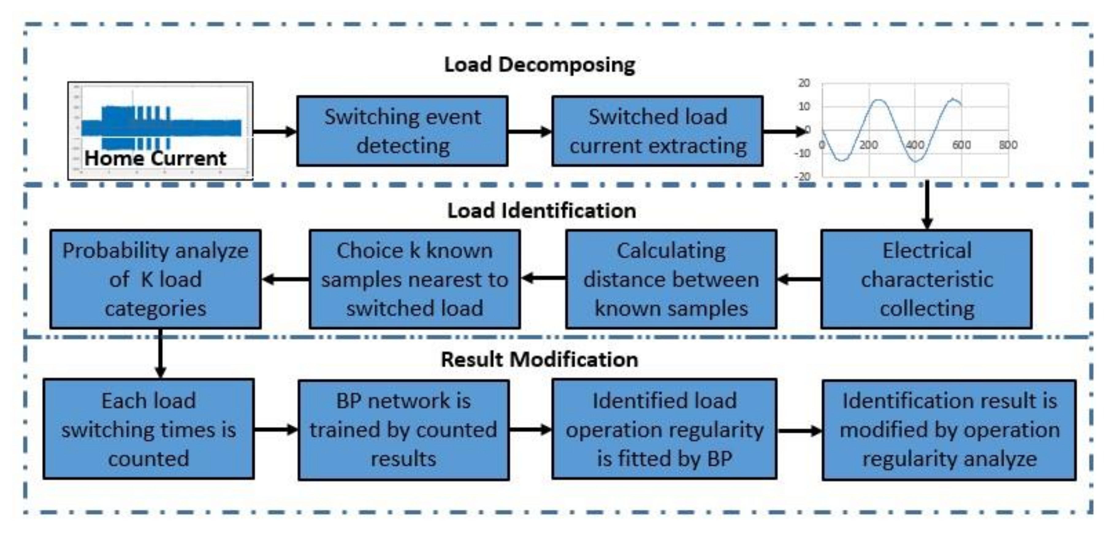
This section introduces the specific process of the proposed method, and Figure 3 demonstrates the overall process.
3.1. Switching Event Detecting and Combined Signal Decomposition
The current paper defines load switching events as electrical events. When an electrical event occurs in a home, the current intensity of the home changes significantly [17]. Indeed, this paper detects electrical events based on the change of current intensity. The home current and voltage are sampled with a certain frequency, and the study records the current and voltage signals within 2 s, so that 2 s is a monitoring period. The current intensity of sampled signals within 2 s can be calculated by Equation (1),
In Equation (1), ʘ is the total number of sampling within 2 s, while is the value of the sampling current. Equation (2) can express the change of current intensity in present monitoring period relative to the previous monitoring period.
In Equation (2), and are current intensity for T and (T − 1) monitoring period, respectively. If the is larger than , the electrical event is occupied, and is the current intensity change judging threshold.
An electrical event is detected, which is caused by load switching, so that one can extract the independently working current of load through Equation (3),
In Equation (3), is the steady current signal recorded after detecting load switching, is the steady current signal been recorded before detecting load switching.
3.2. Load Identification Using KNN Algorithm
The current is decomposed when extracted from a switched load. The decomposed current can be used to identify the type of switched load using a k-nearest neighbors (KNN) algorithm. This process works by first obtaining currents from different known loads and then expanding these currents using Fourier series. The first to fourth harmonics of these currents were used as electrical properties to form a known sample set. The method proposed in Section 3.1 was then used to detect and decompose the current from an unknown load into various signals. The current from the unknown load was also expanded using Fourier series to obtain its electrical properties and form an unknown sample set. The value of k was set in the KNN algorithm [18]. The Euclidean distance between the electrical properties of the known samples and the electrical properties of the unknown samples was measured. The Euclidean distance was measured using Equation (4). The first k known samples nearest to the unknown sample set were selected.
where is the unknown load with number ζ, is the nth sample in the known sample set m, P is the dimension of the sample, and and are the pth coordinates for samples and , respectively.
Finally, Equation (5) was used to calculate the probability of the unknown load belonging to each load category. The load category with the highest probability was assigned to the unknown load.
where is the probability of the decomposed current belonging to the m load category, M is the total number of load categories, Q is the number of samples in k known samples nearest to the unknown sample set that belong to the m load category, and is the reciprocal of the Euclidean distance in Equation (4). The reciprocal of Equation (4) is given by Equation (6).
3.3. Load Identification Based on Electrical Properties and Switching Probabilities
The KNN algorithm is ineffective in load identification where the electrical properties of two or more load categories are similar. This leads to false identification by KNN algorithms. Loads with similar electrical properties have different switching probabilities at any specific time. This study used a back-propagation neural network (BPNN) to fit the distribution curve of the switching probability in the identified load. This curve contained the operation pattern of the identified load. The switching probability of the identified load was then checked against the operation pattern of the identified load, and the identification result was modified if necessary.
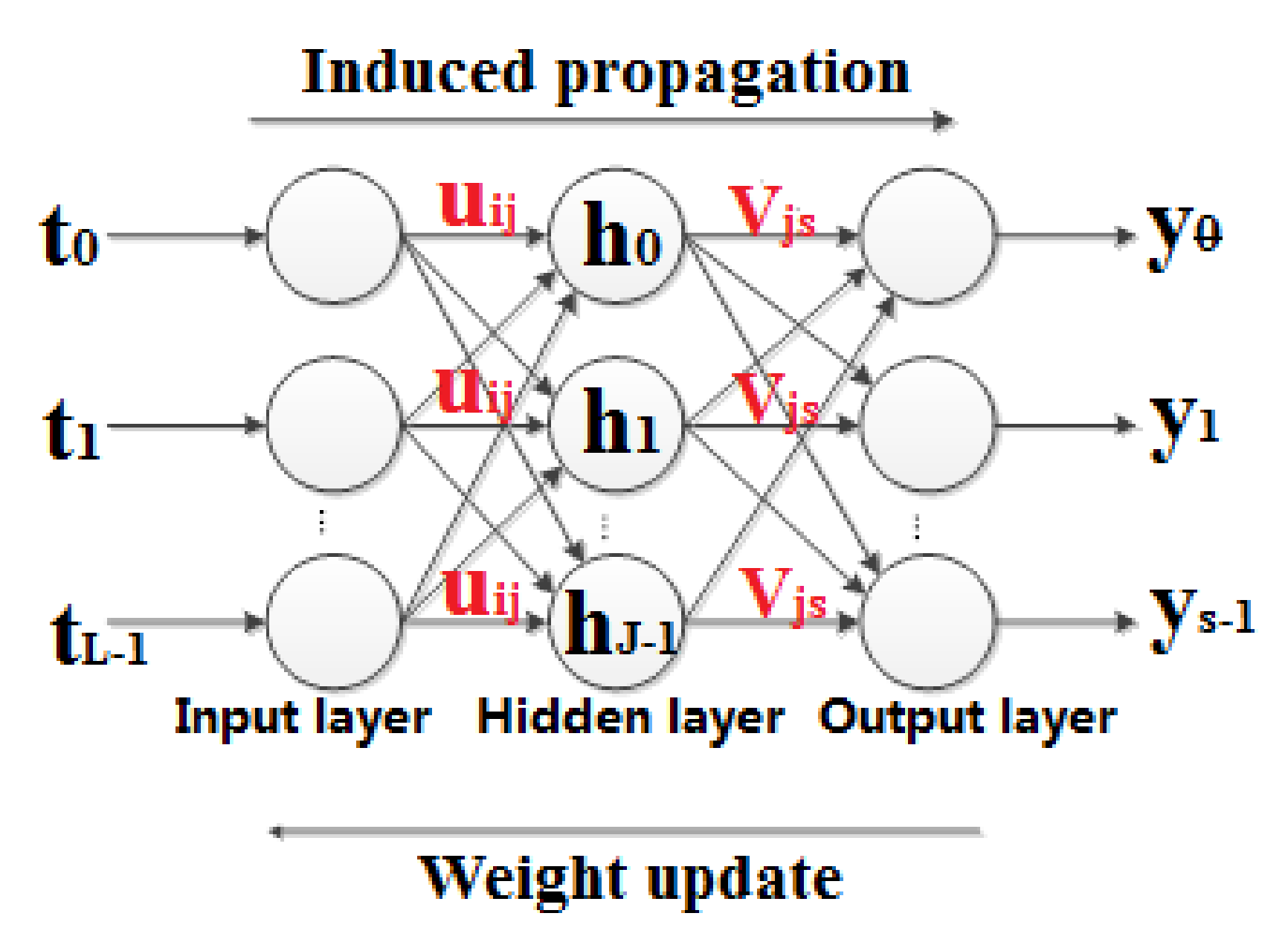
BPNNs generally consist of three layers, namely, the input layer, hidden layer, and output layer. Nodes between layers are connected with neural weights, as shown in Figure 4. BPNN processes induced propagation and weight updates [19]. Regarding processing induced propagation, training data were fed to the BPNN to obtain an induced response. The network error in the BPNN was then obtained by calculating the difference between the expected input data and the induced response. Regarding processing weight updates, the calculated network error was back-propagated from the output layer to the input layer, and the weight of each neuron was updated in order to decrease the network error. This process was repeated until the network error fell within an acceptable pre-determined range.
The data set for BPNN training was built in advance. In this study, a day was divided into 24 periods, with each period being 1 h. The number of appliance switching events in loads during each period was counted, and it formed the data set used to train the BPNN. Four kinds of loads were identified and labeled as known, the corresponding data set is a third-order matrix of 4 × 24 × 2, in which 4 represents the number of different of loads, 24 represents the number of periods, and 2 represents the number of load labels and the number of load switching events in a period. The BPNN used in this study had an input layer, 2 hidden layers, and an output layer. There were 32 neural units in the first hidden layer, and 64 neural units in the second hidden layer.
The process of induced propagation is detailed as follows. The data set was forward-propagated. The 4 × 24 × 2 matrix used as input was multiplied with the 2 × 32 weight matrix of the first hidden layer. The input data set was mapped to the 4 × 24 × 32 features of the first hidden layer, and then nonlinear mapping was performed on the first hidden layer. The output of the first hidden layer was multiplied with the 32 × 64 weight matrix to obtain the 4 × 24 × 64 features of the second hidden layer. Finally, the output of the second hidden layer was multiplied by the 64 × 1 weight matrix to obtain the final 4 × 24 × 1 output of the BPNN. The final output, , is the forecasted number of switching in each period.
Regarding the process of weight updates, the network error was calculated using the difference between the network output and the expected input. The network error was back-propagated. The expected input is the number of load switching events counted during each period. In the actual network training process, a dropout mechanism was added to the second hidden layer to randomly discard some nodes with probabilities of 0.1 in order to improve the generalization of the model. A stochastic gradient descent algorithm [20] was used to adjust the weights in the network. The BPNN training ended when the network error was small enough.
BPNN was used to fit the curve of switching frequency during each time of the day. Therefore, switching times were normalized. The curve of load switching frequency was integrated to obtain the area under the curve. The area under the curve was divided by the switching frequency in each period to form the probability distribution curve of load switching. The probability distribution curve of load switching was treated as a curve of load operation pattern. The load operation pattern was then evaluated. If the operation pattern of the identified load did not match with the corresponding switching probability, the identification result was wrong. The entire process was repeated if the operating pattern of the identified load did not match the corresponding switching probability. Loads with similar operating patterns and switching probabilities were limited. Therefore, the right load category could be found in the k known samples nearest to the unknown sample set.
4. Experiment and Analysis
Experiments were carried out on the measured data of two homes that verify the effectiveness of the proposed method. The measured data within 7 days were collected from two independent homes using acquisition devices. Indeed, the electrical appliances of the home were used as usual during the acquisition process, so the home appliance operation regularity was the same as usual. To verify the algorithm, a data acquisition device was also installed for each home appliance, thereby obtaining the operation regularity of the home appliance and providing a reference for the experiment results. The home voltage is 220 V, and the sample frequency of each acquisition device is 10 kHz. The home appliance includes one TV (TV), one refrigerator (RE), one microwave oven (MO), two air conditioners (AC-A and AC-B), two laptops (LAP-A and LAP-B) and two electric kettles (EK-A and EK-B). The second home appliance includes one TV(TV), one refrigerator (RE), one microwave oven (MO), one air conditioner (AC-C), one laptop (LAP-C), one rice cooker(RC) and one sterilizer (STE).
4.1. Verification of Signal Decomposition Effect
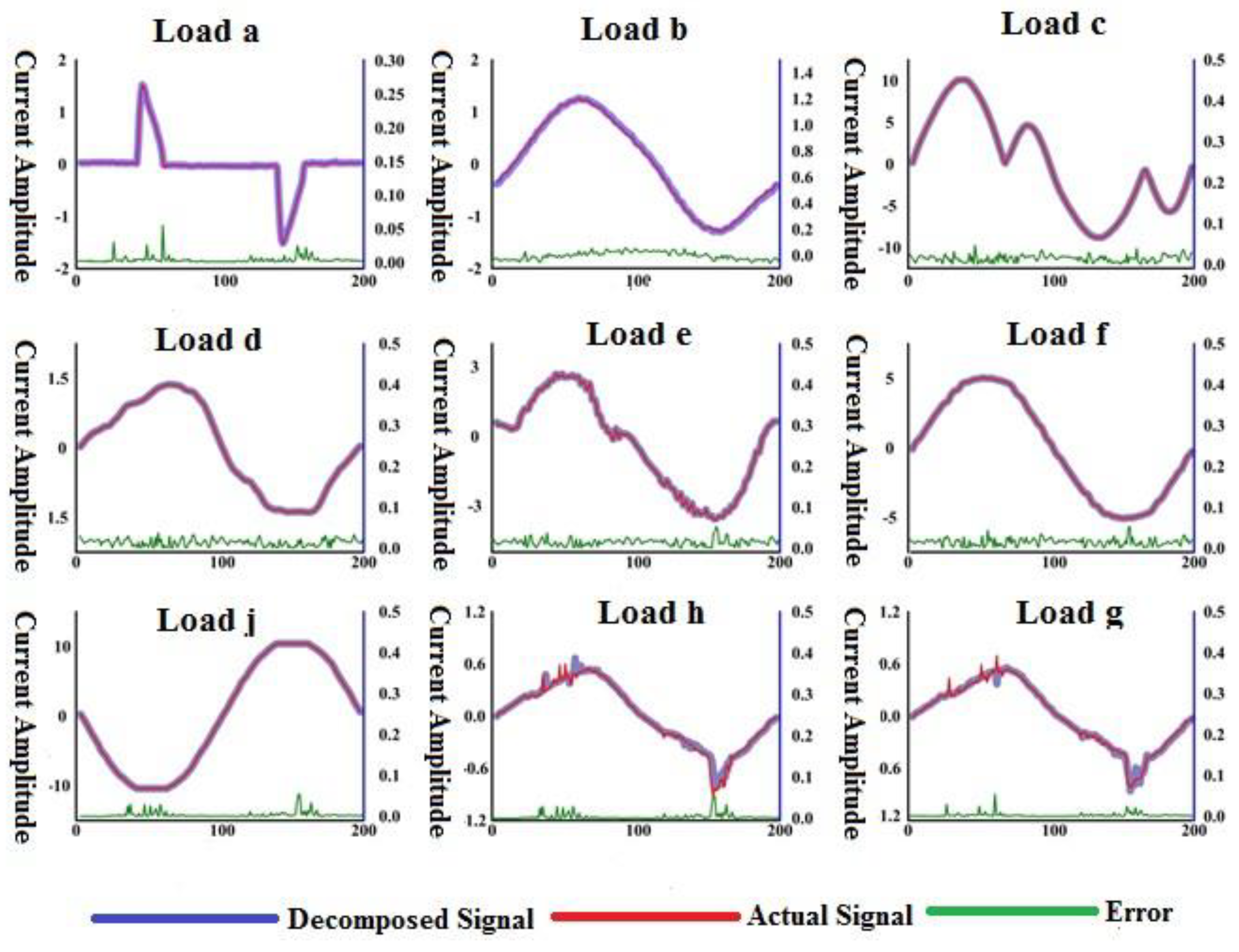
Figure 5 shows: the independently working current signal decomposed from complex home current signals, the actual current signal was directly collected by the acquisition device at the load side, and the error between the decomposed current signal and the actual current signal.
The two signals in Figure 5 are almost identical and the error is small between the two signals. This means that the proposed algorithm can effectively extract the independent load working current from mix home current signal.
Table 1 shows the similarity coefficient and root mean square error between the decomposed signal and the actual signal in first home. As Table 1 indicates, the similarity coefficients are higher than 0.9, and the average similarity coefficient is 0.9477. Furthermore, the mean square error between two signals is lower than 0.5, and the average mean square error is 0.305, proving that the proposed method effectively decomposes signals. The load characteristic is totally contained in the decomposed signal. Equations (7) and (8) calculate the similarity coefficient R and root mean square error (RMSE):
In Equations (7) and (8), and are the decomposed current and the actual current, respectively. and are the standard deviation for decomposed current and actual current, respectively.
Table 2 shows the similarity coefficient and root mean square error between the decomposed signal and the actual signal in the second home. As Table 2 indicates, the similarity coefficients are higher than 0.96, and the mean square error between two signals is lower than 0.02, proving that the proposed method effectively decomposes signals for different homes.
4.2. Verification of Initial Load Identification
The working current signal of the switched load was decomposed and extracted, the working current signal was initially identified by the KNN algorithm. The number of k in the KNN algorithm was set as five. The harmonic of load working current was treated as a characteristic dimension to calculate the Euclidean distance of the electrical characteristic. Table 3 shows the first to fourth harmonics of six home appliances which are known samples in KNN.
The first to fourth harmonic current amplitudes of the unknown load, obtained by the load decomposition method, were used as the clustering center, and the Euclidean distance between the known load sample set and the cluster center was calculated to realize the initial identification.
Table 4 shows the types of home appliances involved in this paper, along with minimum and average Euclidean distance of the electrical characteristics between the decomposed load working current and five known samples. Table 4 shows that unknown load one is the television, unknown three is the microwave oven, and the other identification results are obtainable by following the probability of the Euclidean distance.
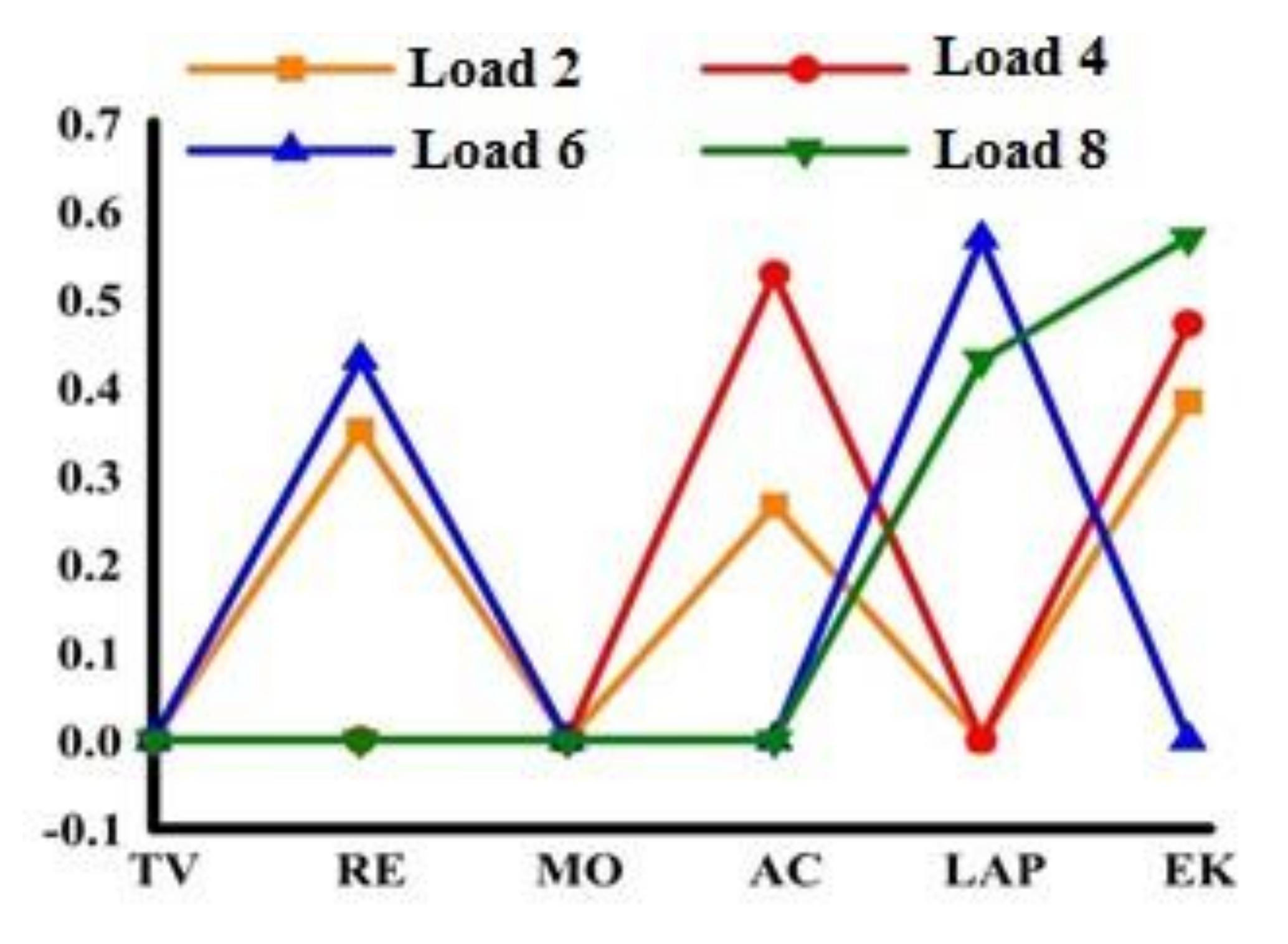
Figure 6 shows the identification results of unknown loads two, four, six and eight, which are achieved through probability. Figure 6 indicates unknown loads two, four, six and eight as being the electric kettle, air conditioner, notebook computer and electric kettle, respectively.
Table 5 shows the identification result. According to the Table 5, unknown loads from one to seven were identified as RE, TV, MO, AC, LAP and RC, respectively. The unknown loads six and seven were both identified as RC, but can also be identified as SET, which produces mistakes in the identification result, the mistake will be corrected in modification step.
4.3. Verification of Modification Method
The electrical characteristic of decomposed current one is nearest to the TV, so the switched load was identified as TV, and it switched two times at 1pm. This data set trains the BP network. The trained BP network can fit the switching probability distribution curve of the TV.
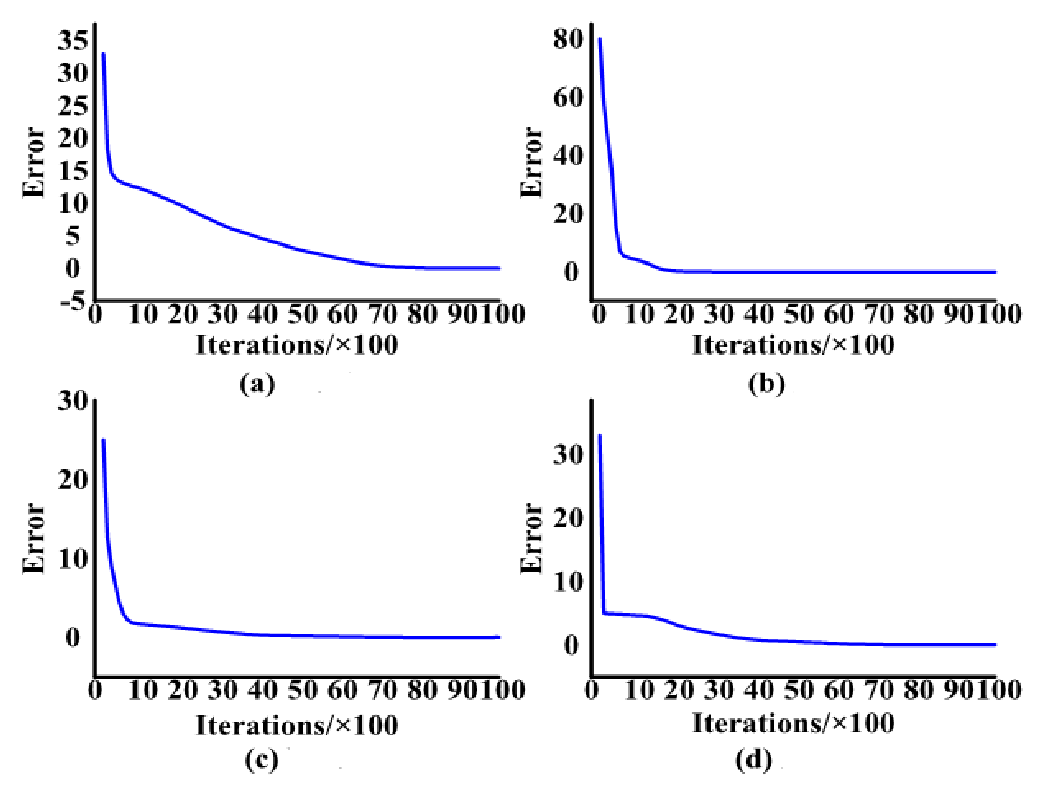
Considering the mentioned example, four load switching times in the specific period are used to train the BP network. In the training process, the parameters of the BP neural network include the number of hidden layers (Nhl), the number of neurons in each hidden layer (Nneu1 and Nneu2), the initial learning rate, iteration times and dropout rate in Table 6. Figure 7 shows the training process, while the network error decreases alongside increases in iteration times in the training process. When iterations times reach 10,000, the error of the four BP networks is close to zero, meaning the training of BP has concluded.
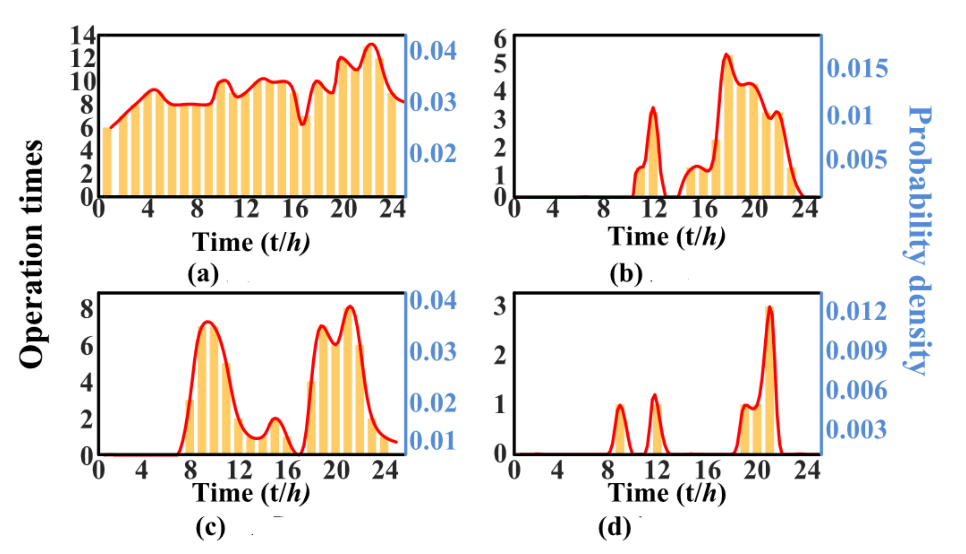
If the BP network finished the training, the load switching time distribution curve fitted by BP is near to the expected value. The identified result was input into the BP network to fit the switching probability distribution curve of the identified load. Figure 8′s histogram indicates the switching times of the identified home appliances at each hour of the day. The switching probability distribution curve fitted by the BP neural network is close to the actual situation.
The current study obtained the switching probability distribution curves of identified home appliances. The abscissa is 24 h in day and the ordinate is the probability density. Therefore, the probability of the appliance used in each hour period is the area under the curve within the corresponding time period.
Firstly, one must analyze the EK-1, which is used all day, and the operation period is very regular. Normally, the hot pot is only used during a specific period of time rather than all day. Therefore, the switching probability distribution curve is not a hot pot; it can be judged that the load identification under the KNN algorithm is incorrect. According to the modification, the load should be classified as the refrigerator, because the refrigerator has the second highest probability in load identification part. Additionally, the time period of the refrigerator operation is consistent with the fitted the switching probability distribution curve.
Secondly, one must analyze the AC. According to the switching probability distribution curve, the air conditioner is mainly used at noon and at night, which is consistent with the normal operation conditions of the consumer. Indeed, the load identification result is correct.
Thirdly, the LAP was analyzed due to the switching probability distribution curve. Notebook computers are mainly used from 8 a.m. to 12 a.m. in the morning and 19 p.m. to 23 p.m. in the evening, which is consistent with the normal conditions. Accordingly, the result of load identification is correct. Finally, EK-2 requires analysis.
According to the distribution curve, the hot pot is always used in the morning, noon and evening, and is not used in other periods, which is consistent with the normal condition.
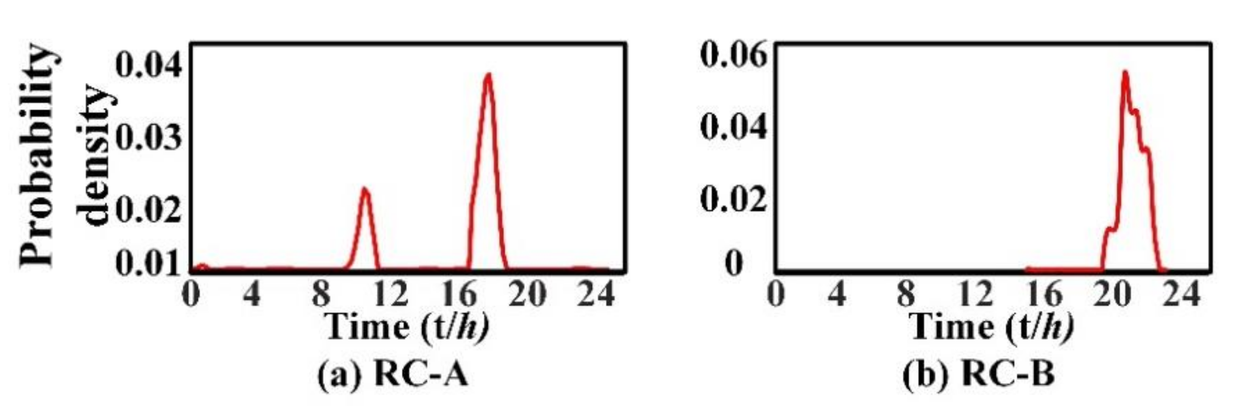
Figure 9 shows the switching probability distribution curve of two loads identified as the rice cooker in family two. It can be seen from the figure that the probability of RC-A running between 8:00 to 12:00 and 16:00 to 19:00 is relatively high, and these two periods are usually before lunch or dinner, which is consistent with the conditions of the normal user, so it can be judged that the identification result is correct. In contrast, the running time of RC-B is always from 20:00 to 23:00 p.m., which is generally after dinner, it is obviously inconsistent with the living habits, so it can be considered that the load identification has been misjudged, the identification result needs to be modified. By comparing with the data obtained by the independent data acquisition device, we can know that the load is indeed the disinfection cabinet. Therefore, the probability distribution curve of different loads can provide a reliable basis for the identification of similar load characteristics.
4.4. Comparison with Existing Algorithms
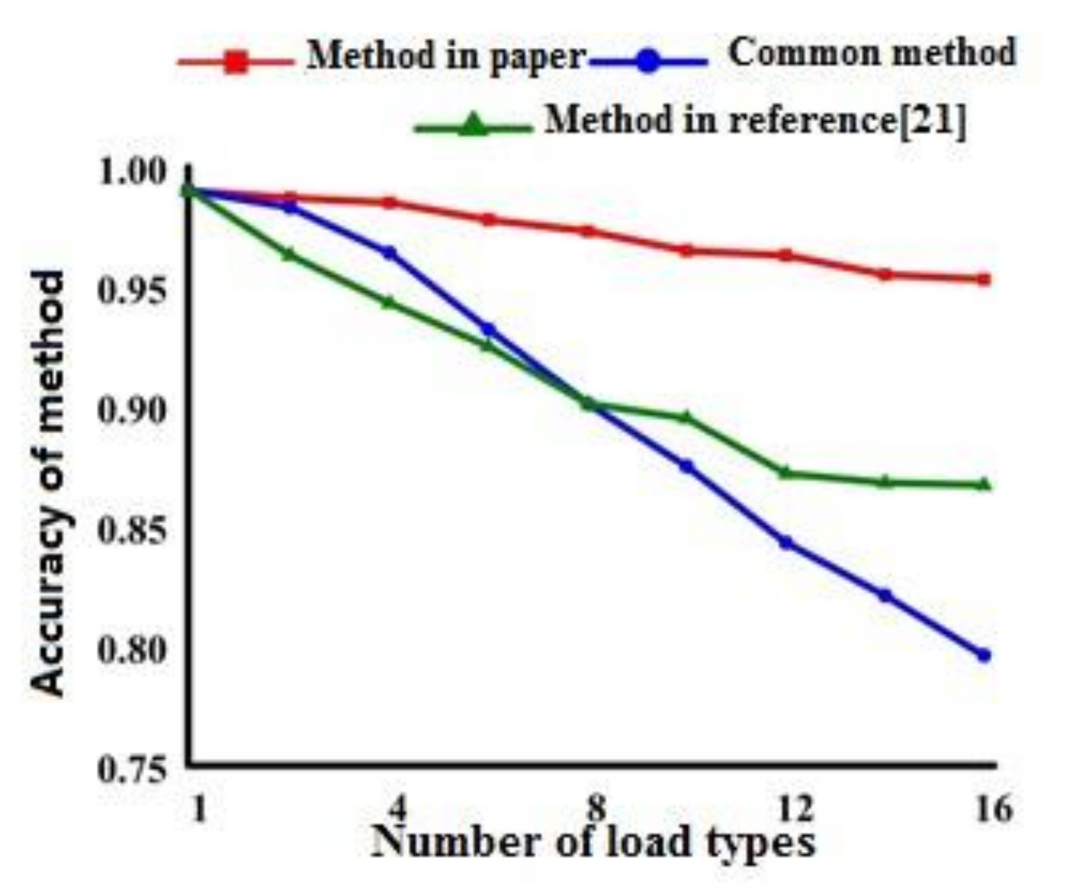
This paper uses the KNN algorithm to initially identify the unknown load. The common method only identifies loads based on various electrical characteristics, which is the final identification result. Furthermore, the BP neural network fits the switching frequency of different loads to obtain the load switching probability distribution curve. The initial identification of the load only provides a data bank for the modification step, so this paper selected the commonly used KNN algorithm to identify the load. As an important part of this paper, the process of load switching frequency, a BP neural network is used, which is not involved in traditional work. Compared with the method mentioned in this paper, the algorithm performance in reference [21] performed Fourier transform on the current and treats harmonic as the feature to identify the load.
Figure 10 reveals a comparison of identification accuracy rate between the modified identification result and initial identification result. The accuracy of load identification was effectively improved following modification.
With the improvement of the load type number, the influence for the proposed method is less and the accuracy rate is higher. Indeed, the accuracy rate has been improved.
5. Conclusions
To solve the problem of low identification accuracy of load with similar characteristics in NILM, the current project studied an identification result modification method based on a load switching probability distribution curve. This method focused on the difference in switching probabilities of loads with similar electrical characteristics; this achieved modification of initial load identification. Firstly, the paper used the algorithm for switching event detection and signal decomposition to obtain the independently working current signal of the unknown switched load from the collected current signal. Based on the KNN algorithm, the harmonics of current signal were then taken as the load characteristics to complete the initial load identification. Secondly, based on the initial identification results, the switching times of the load at each hour of the week were fitted to the BP network. Moreover, the switching probability distribution curve of the identified load was obtained. Finally, due to the switching probability distribution curve of the load, the study obtained the load operation regularity. By judging the load operation regularity as reasonable or not, the study modified the identification results.
The experimental data shows that the proposed method effectively improves the accuracy of load identification, and the identification accuracy is higher than 96%. One can verify the improvement of the proposed method by comparing the existing algorithms. By analyzing load operation regularity, the paper modified the initial identification results, thereby providing the new ideal for load identification with similar characteristics.
Future research will quantify the load operation regularity and propose a unified standard to lay the foundation for the automatic implementation of the algorithm.
Author Contributions
Conceptualization; methodology; validation; writing—original draft preparation—S.W.; writing—review and editing—K.L.L. All authors have read and agreed to the published version of the manuscript.
Funding
This research received no external funding.
Conflicts of Interest
The authors declare no conflict of interest.
References
- Zeng, M.; Shi, L.; He, Y. Status, challenges and countermeasures of demand-side management development in China. Renew. Sustain. Energy Rev. 2015, 47, 284–294. [Google Scholar]
- Wu, C.; Zhang, H.; Hou, Y.; Cao, L.; Liu, F. Analysis of Binjin UHVDC restart failure and relevant suggestions on secure and stable operation of power grid. Energy Procedia 2018, 145, 452–457. [Google Scholar]
- Hart, G. Nonintrusive appliance load monitoring. Proc. IEEE 1992, 80, 1870–1891. [Google Scholar]
- Hong, Y.; Chou, J.J. Nonintrusive energy monitoring for microgrids using hybrid self-organizing feature-mapping networks. Energies 2012, 5, 2578–2593. [Google Scholar]
- Figueiredo, M.; De Almeida, A.; Ribeiro, B. Home electrical signal disaggregation for non-intrusive load monitoring (NILM) systems. Neurocomput 2012, 96, 66–73. [Google Scholar]
- Jian, L.; Ng, S.; Kendall, G.; Cheng, J. Load Signature Study-Part I: Basic Concept, Structure, and Methodology. IEEE Trans. Power Deliv. 2010, 25, 551–560. [Google Scholar]
- Semwal, S.; Singh, M.; Prasad, R.S. Group control and identification of residential appliances using a nonintrusive method. Turk. J. Electr. Eng. Comput. Sci. 2015, 23, 1805–1816. [Google Scholar]
- Chang, H.; Chen, K.; Tsai, Y.; Lee, W. A new measurement method for power signatures of nonintrusive demand monitoring and load identification. IEEE Trans. Ind. Appl. 2012, 48, 764–771. [Google Scholar]
- Chang, H.; Yang, H. Applying a non-intrusive energy-management system to economic dispatch for a cogeneration system and power utility. Appl. Energy 2009, 86, 2335–2343. [Google Scholar]
- Chang, H. Genetic algorithms and non-intrusive energy management system based economic dispatch for cogeneration units. Energy 2011, 36, 181–190. [Google Scholar]
- Srinivasan, D.; Ng, W.S.; Liew, A.C. Neural-network-based signature recognition for harmonic source identification. IEEE Trans. Power Deliv. 2006, 21, 398–405. [Google Scholar]
- Ruzzelli, A.G.; Nicolas, C.; Schoofs, A.; O’Hare, G.M.P. Real-time recognition and profiling of appliances through a single electricity sensor. In Proceedings of the 7th Annual IEEE Communications Society Conference on Sensor: Mesh and Ad Hoc Communications and Networks (SECON), Boston, MA, USA, 21–25 June 2010; pp. 1–9. [Google Scholar]
- Gabaldo’n, A.; Molina, R.; Mari’n-Parra, A.; Valero-Verdu’, S.; A’lvarez, C. Residential end-uses disaggregation and demand response evaluation using integral transforms. J. Mod. Power Syst. Clean Energy 2017, 5, 91–104. [Google Scholar]
- Hassan, T.; Javed, F.; Arshad, N. An empirical investigation of V-I trajectory based load signatures for non-intrusive load monitoring. IEEE Trans. Smart Grid 2013, 5, 870–878. [Google Scholar]
- He, D.; Du, L.; Yang, Y.; Harley, R.; Habetler, T. Front-end electronic circuit topology analysis for model-driven classification and monitoring of appliance loads in smart buildings. IEEE Trans. Smart Grid 2012, 4, 2286–2293. [Google Scholar]
- Rahimpour, A.; Qi, H.; Fugate, D.; Kuruganti, T. Non-intrusive energy disaggregation using non-negative matrix factorization with sum-to-k constraint. IEEE Trans. Power Syst. 2017, 32, 4430–4441. [Google Scholar]
- Wu, X.; Jiao, D.; Liang, K.; Han, X. A fast online load identification algorithm based on V-I characteristics of high-frequency data under user operational constraints. Energy 2019, 188, 116012. [Google Scholar]
- Wen, X.; Lu, G.; Liu, J.; Yan, P. Graph modeling of singular values for early fault detection and diagnosis of rolling element bearings. Mech. Syst. Signal Process. 2020, 145, 106956. [Google Scholar]
- Yu, F.; Xu, X. A short-term load forecasting model of natural gas based on optimized genetic algorithm and improved BP neural network. Appl. Energy 2014, 134, 102–113. [Google Scholar]
- Peng, Y.; Hao, Z.; Yun, X. Lock-Free Parallelization for Variance-Reduced Stochastic Gradient Descent on Streaming Data. IEEE Trans. Parallel Distrib. Syst. 2020, 31, 2220–2231. [Google Scholar]
- Ahmadi, H.; Marti, J.R. Load Decomposition at Smart Meters Level Using Eigenloads Approach. IEEE Trans. Power Syst. 2015, 30, 3425–3436. [Google Scholar]
Figure 1.
- Loads working current wave and loads operation period.

Figure 2.
Overall structure of non-intrusive load monitoring (NILM).

Figure 3.
Process of the NILM method. BP: back propagation.

Figure 4.
Structure of the back-propagation neural network (BPNN).

Figure 5.
Comparison between decomposed signal and the actual signal in first home.

Figure 6.
Probability of Euclidean distance.

Figure 7.
Network error tendency curve of EK-1 (a), AC (b), LAP (c) and EK-2 (d).

Figure 8.
Load switching probability distribution curve in first home for EK-1 (a), AC (b), LAP (c) and EK-2 (d).
Figure 8.
Load switching probability distribution curve in first home for EK-1 (a), AC (b), LAP (c) and EK-2 (d).

Figure 9.
Load switching probability distribution curve for RC-A (a) and RC-B (b).

Figure 10.
Comparison between the two methods.


Table 1.
Similarity coefficient and root mean square error (RMSE) between the decomposed signal and the actual signal in first home.
Table 1.
Similarity coefficient and root mean square error (RMSE) between the decomposed signal and the actual signal in first home.
| Decomposed Current | R | RMSE |
|---|---|---|
| No. 1 | 0.941 | 0.389 |
| No. 2 | 0.903 | 0.521 |
| No. 3 | 0.994 | 0.029 |
| No. 4 | 0.982 | 0.076 |
| No. 5 | 0.975 | 0.113 |
| No. 6 | 0.936 | 0.452 |
| No. 7 | 0.927 | 0.417 |
| No. 8 | 0.918 | 0.458 |
| No. 9 | 0.953 | 0.289 |
Table 2.
Similarity coefficient and RMSE between the decomposed signal and the actual signal in second home.
Table 2.
Similarity coefficient and RMSE between the decomposed signal and the actual signal in second home.
| Decomposed Current | R | RMSE |
|---|---|---|
| No. 1 | 0.997 | 0.0032 |
| No. 2 | 0.963 | 0.0127 |
| No. 3 | 0.994 | 0.0092 |
| No. 4 | 0.992 | 0.0077 |
| No. 5 | 0.965 | 0. 0182 |
| No. 6 | 0.986 | 0.0176 |
| No. 7 | 0.997 | 0.0098 |
Table 3.
1st to 4th harmonic of six home appliance.
| Home Appliance | 1st Harmonic | 2nd Harmonic | 3rd Harmonic | 4th Harmonic |
|---|---|---|---|---|
| TV | 0.345 | 0.009 | 0.310 | 0.008 |
| RE | 1.205 | 0.033 | 0.079 | 0.007 |
| MO | 7.620 | 0.682 | 2.943 | 0.103 |
| AC | 4.477 | 0.691 | 0.334 | 0.187 |
| LAP | 2.769 | 0.172 | 0.432 | 0.272 |
| EK | 5.146 | 0.005 | 0.089 | 0.001 |
Table 4.
Euclidean distance between the decomposed current and 5 known samples.
| TV | RE | MO | AC | LAP | EK | |
|---|---|---|---|---|---|---|
| Decomposed current 1 | 0.131/0.078 | 0 | 0 | 0 | 0 | 0 |
| Decomposed current 2 | 0 | 0.118/0.109 | 0 | 0.156/0.156 | 0 | 0.108/0.095 |
| Decomposed current 3 | 0 | 0 | 0.103/0.086 | 0 | 0 | 0 |
| Decomposed current 4 | 0 | 0 | 0 | 0.108/0.079 | 0 | 0.132/0.122 |
| Decomposed current 5 | 0 | 0.143/0.112 | 0 | 0.118/0.074 | 0 | 0 |
| Decomposed current 6 | 0 | 0.133/0.133 | 0 | 0 | 0.101/0.089 | 0 |
| Decomposed current 7 | 0 | 0.132/0.132 | 0 | 0 | 0.117/0.086 | 0 |
| Decomposed current 8 | 0 | 0 | 0 | 0 | 0.148/0.148 | 0.112/0.101 |
| Decomposed current 9 | 0 | 0 | 0 | 0 | 0.140/0.1140 | 0.108/0.086 |
Table 5.
Initial load identification of the second home.
| TV | RE | MO | AC | LAP | RC | STE | |
|---|---|---|---|---|---|---|---|
| Decomposed current 1 | 0 | 0.681 | 0 | 0.319 | 0 | 0 | 0 |
| Decomposed current 2 | 1 | 0 | 0 | 0 | 0 | 0 | 0 |
| Decomposed current 3 | 0 | 0 | 1 | 0 | 0 | 0 | 0 |
| Decomposed current 4 | 0 | 0.221 | 0 | 0.779 | 0 | 0 | 0 |
| Decomposed current 5 | 0 | 0.125 | 0 | 0 | 0.875 | 0 | 0 |
| Decomposed current 6 | 0 | 0 | 0 | 0.112 | 0 | 0.453 | 0.435 |
| Decomposed current 7 | 0 | 0 | 0 | 0.075 | 0 | 0.505 | 0.420 |
Table 6.
The BP neural network parameters.
| Parameter | Value | Parameter | Value |
|---|---|---|---|
| Nhl | 2 | Initial learning rate | 0.0001 |
| Nneu1 | 32 | Epochs | 10,000 |
| Nneu2 | 64 | Dropout Rate | 0.1 |
Publisher’s Note: MDPI stays neutral with regard to jurisdictional claims in published maps and institutional affiliations. |
© 2020 by the authors. Licensee MDPI, Basel, Switzerland. This article is an open access article distributed under the terms and conditions of the Creative Commons Attribution (CC BY) license (http://creativecommons.org/licenses/by/4.0/).
Share and Cite
MDPI and ACS Style
Wu, S.; Lo, K.L. Non-Intrusive Monitoring Algorithm for Resident Loads with Similar Electrical Characteristic. Processes 2020, 8, 1385. https://0-doi-org.brum.beds.ac.uk/10.3390/pr8111385
AMA Style
Wu S, Lo KL. Non-Intrusive Monitoring Algorithm for Resident Loads with Similar Electrical Characteristic. Processes. 2020; 8(11):1385. https://0-doi-org.brum.beds.ac.uk/10.3390/pr8111385
Chicago/Turabian StyleWu, Sheng, and Kwok L. Lo. 2020. "Non-Intrusive Monitoring Algorithm for Resident Loads with Similar Electrical Characteristic" Processes 8, no. 11: 1385. https://0-doi-org.brum.beds.ac.uk/10.3390/pr8111385
Note that from the first issue of 2016, this journal uses article numbers instead of page numbers. See further details here.